(!) Essential for Python for AI & ML

(*C’est cool ce manuel! J’en extrait ici des infos qui précisent des connaissances acquises!

Une excellente synthèse! *)

Dans Jupyter, si on tape import <TAB>… on obtient la liste des Modules installables.

Statistical Methods and Models

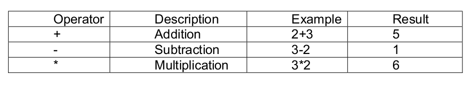
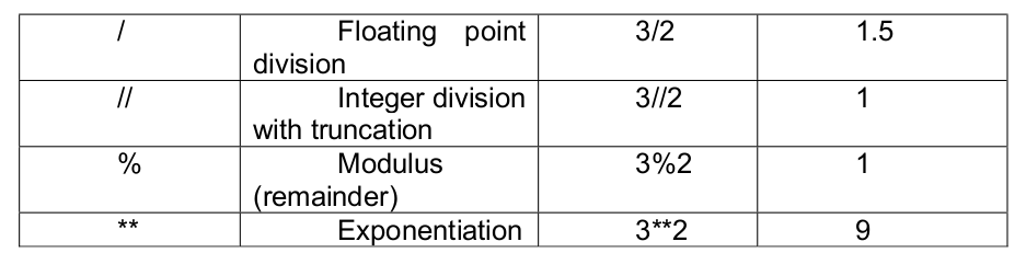
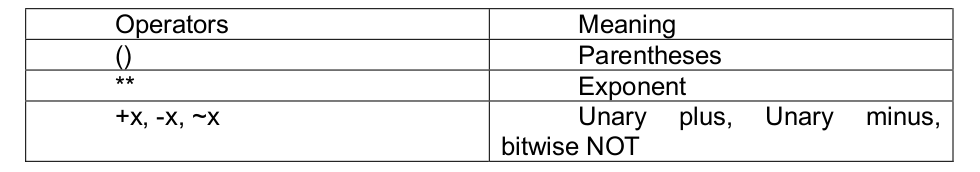
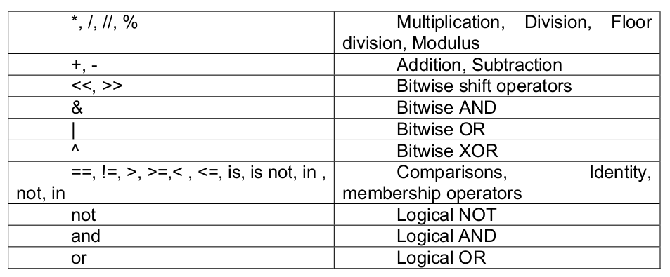
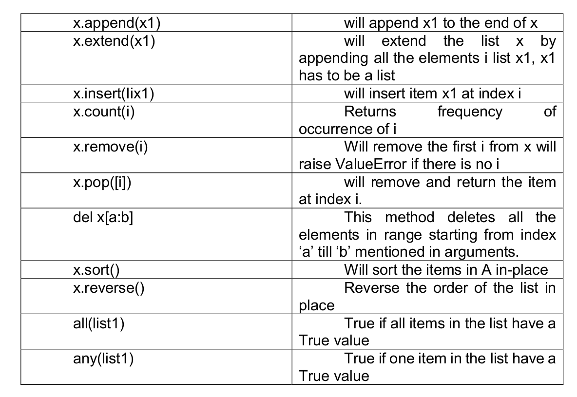
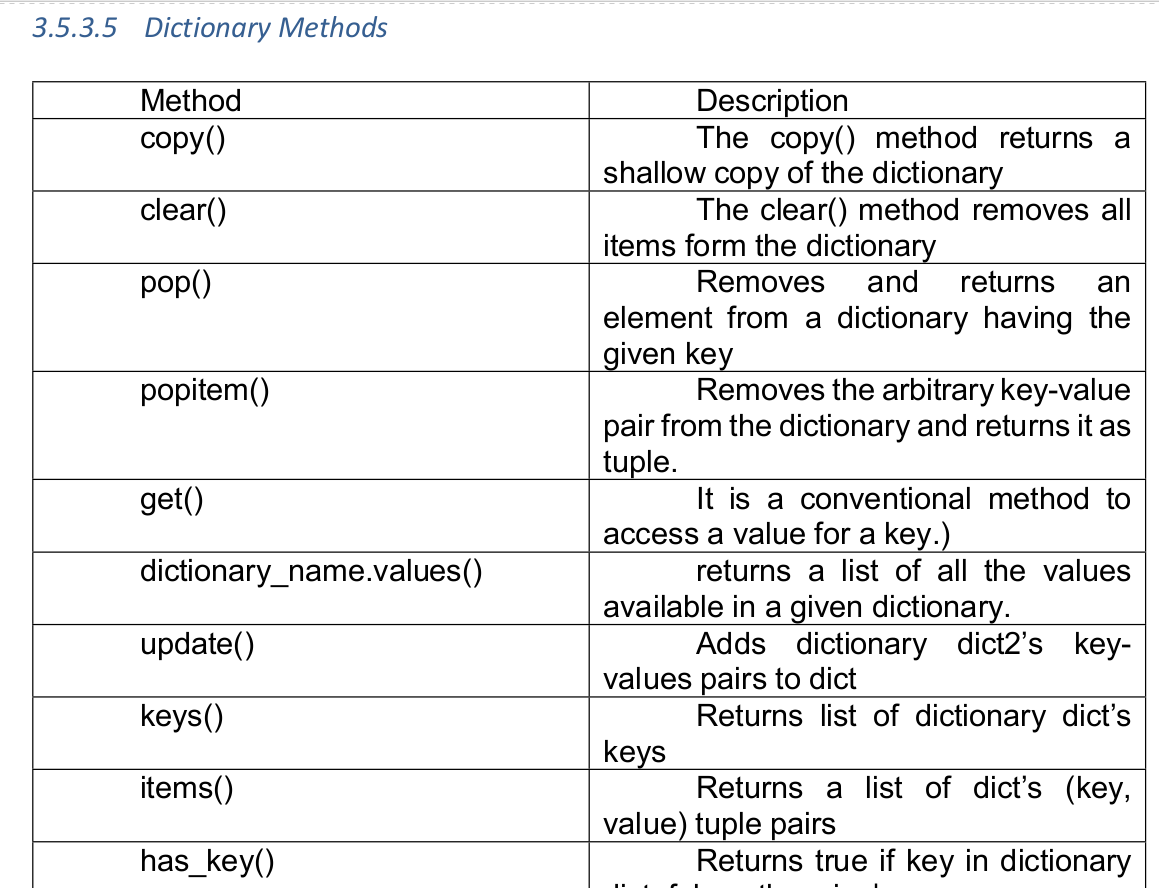
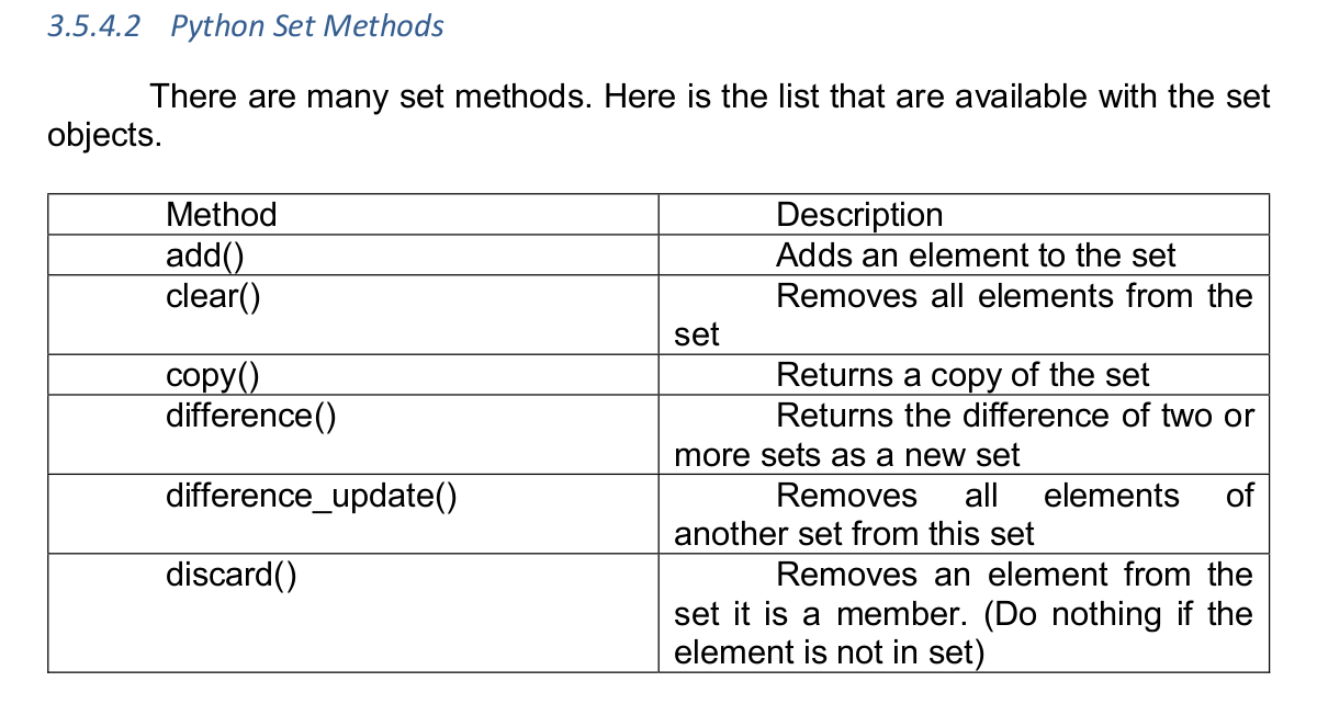
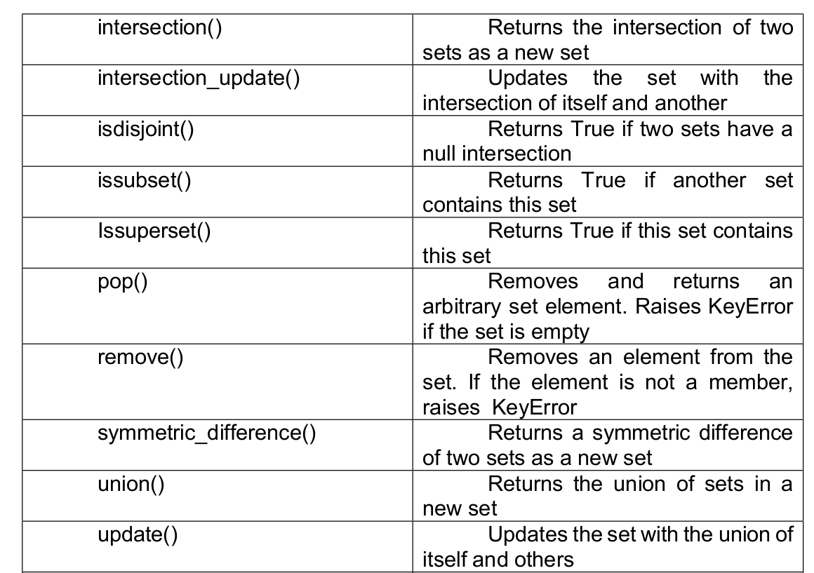
Essential Python

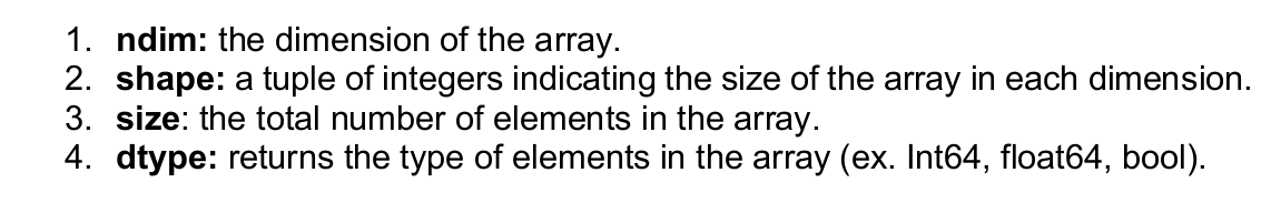
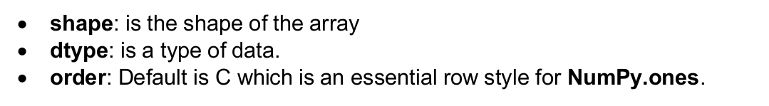
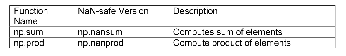
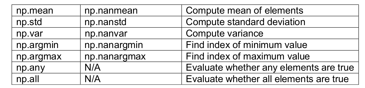
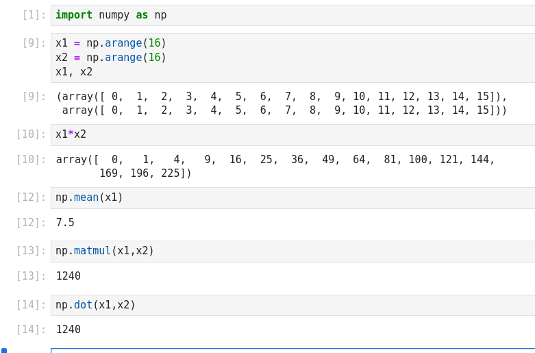
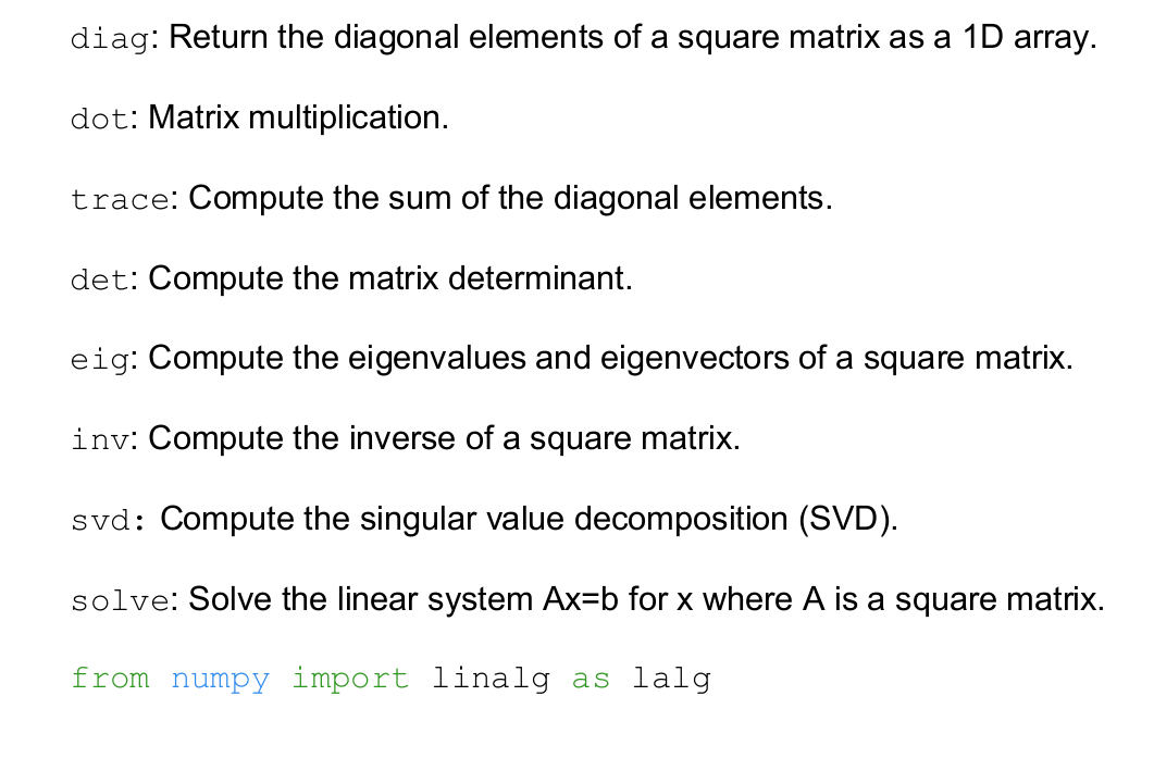
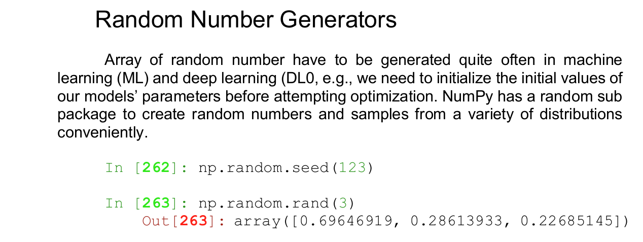
Essential of NumPy

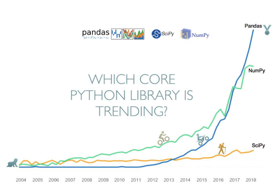
Essential Pandas

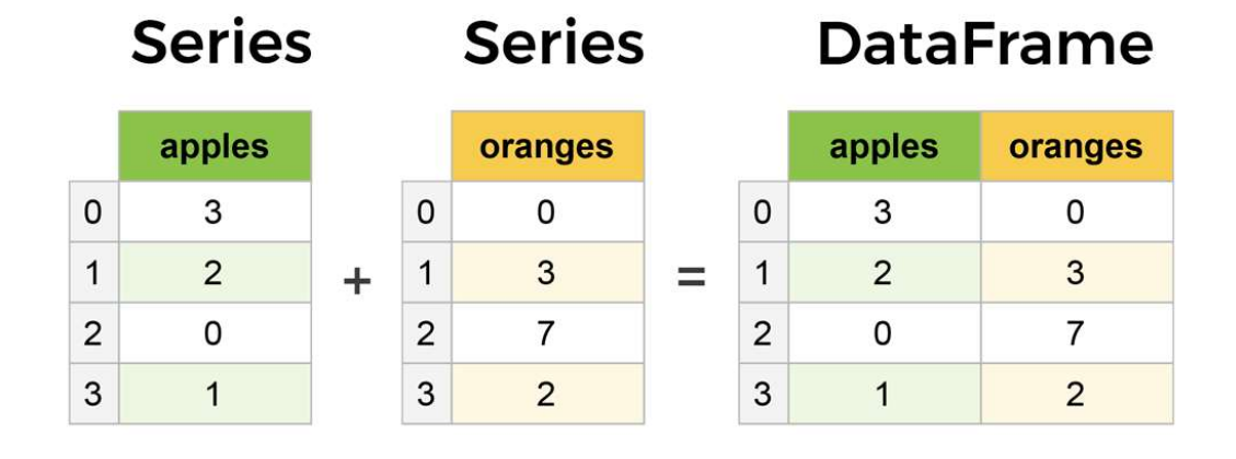
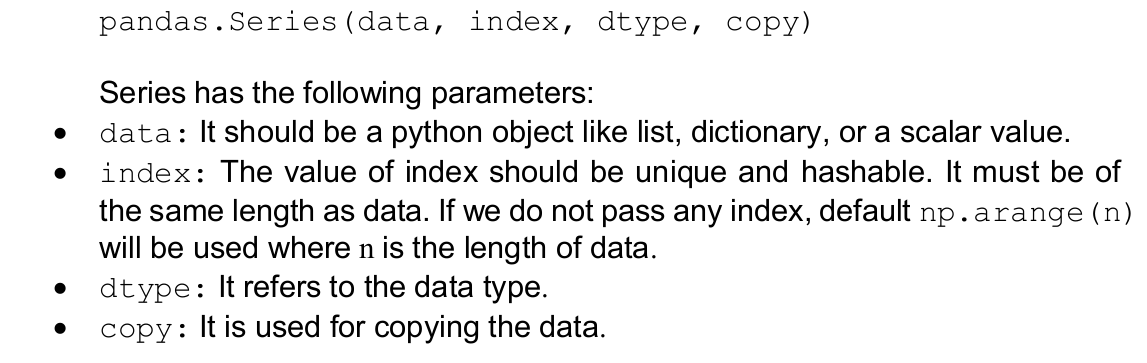
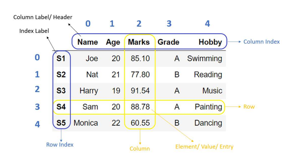
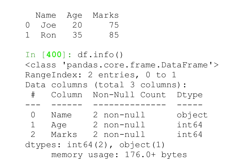
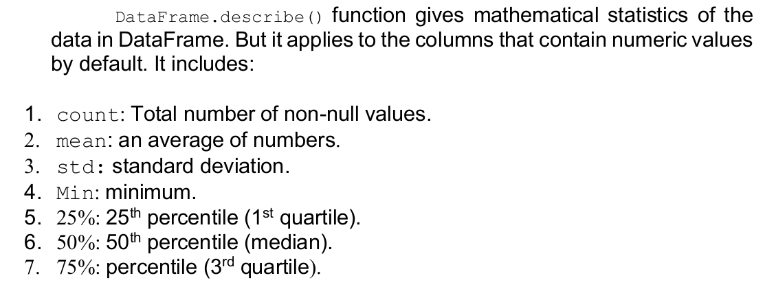
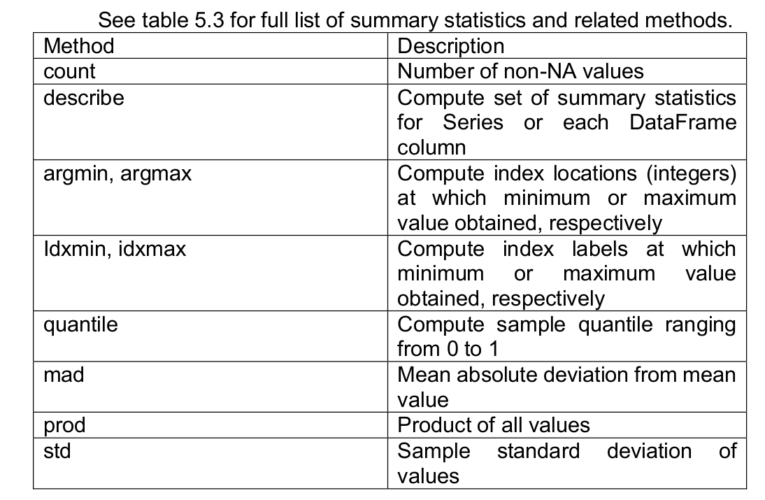
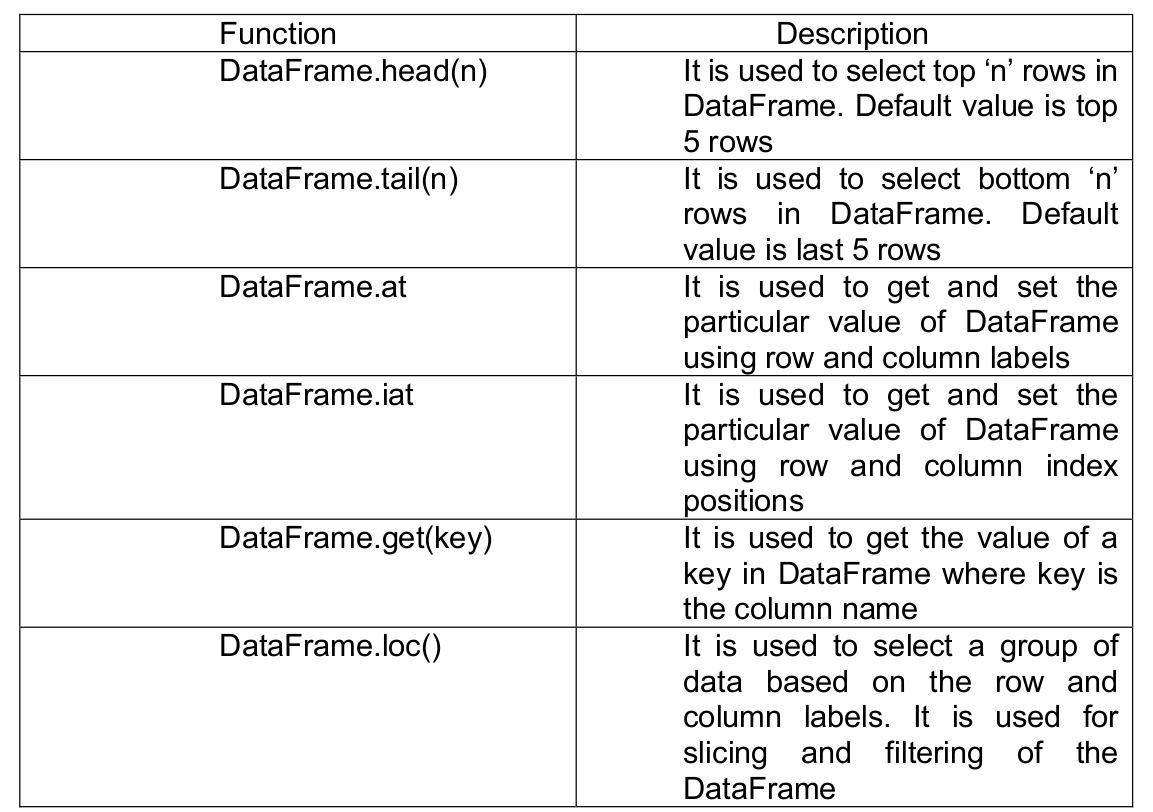
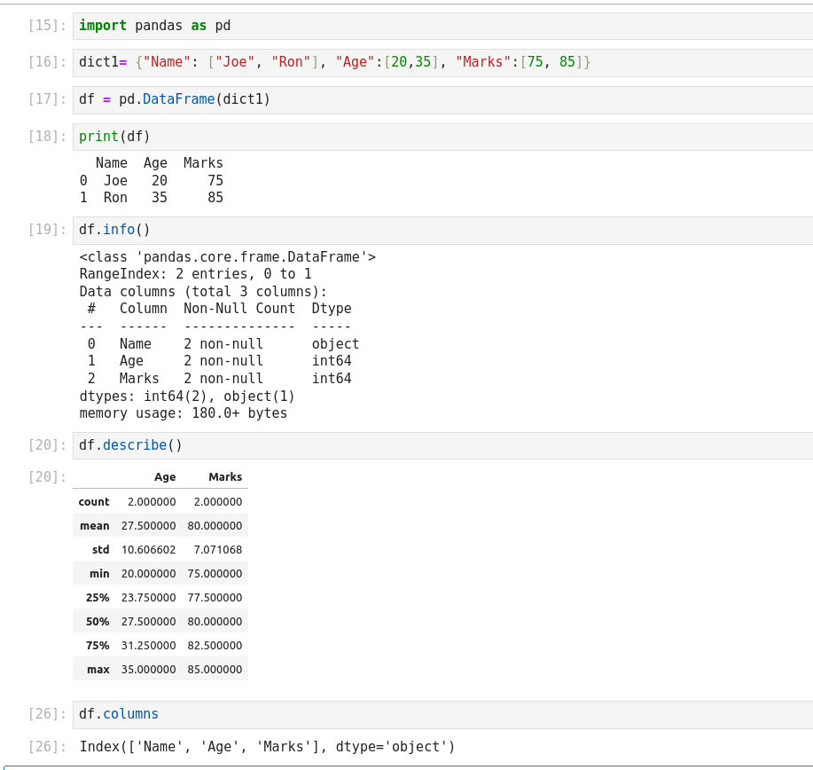
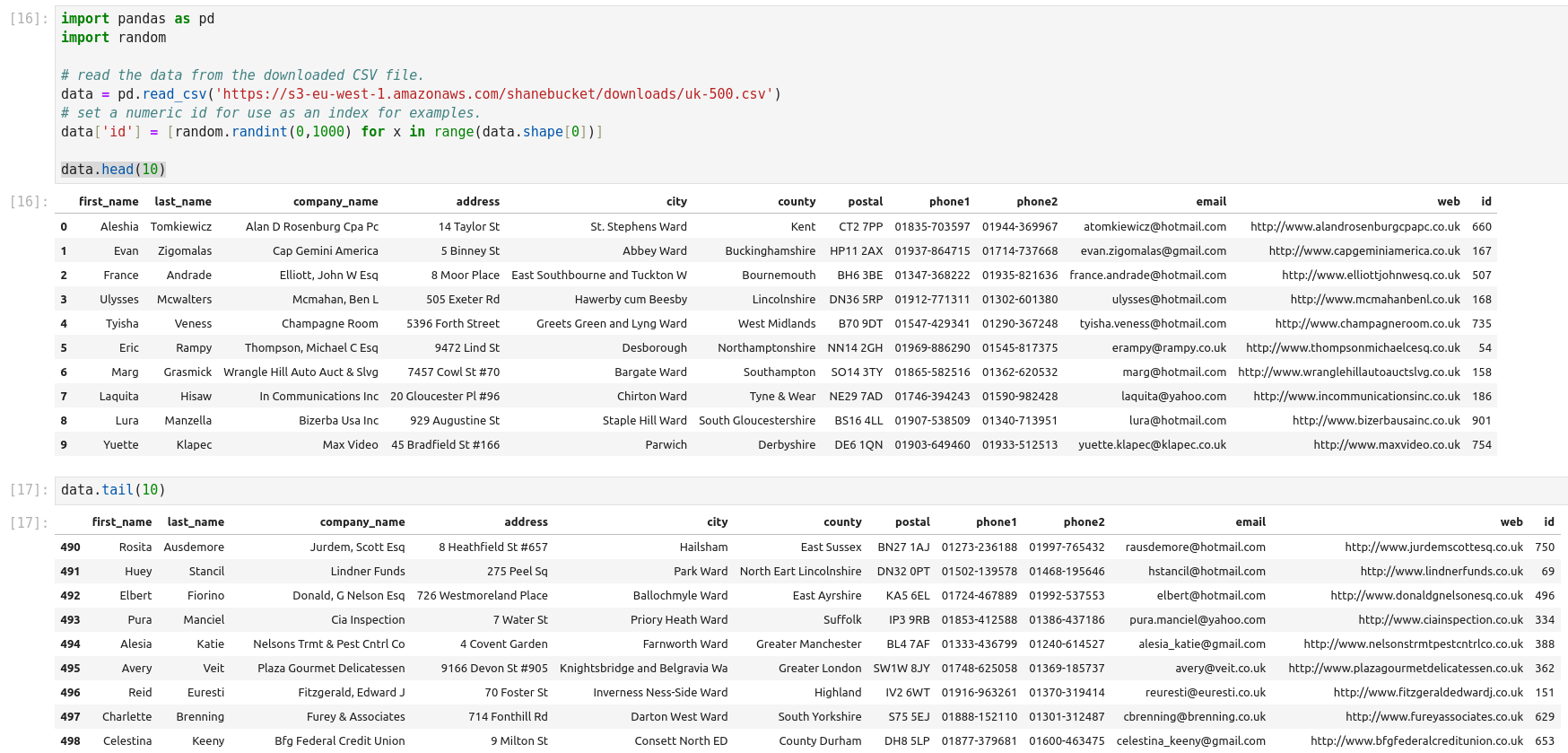
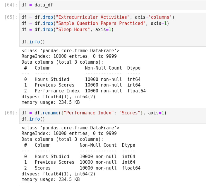
Pandas DataFrame

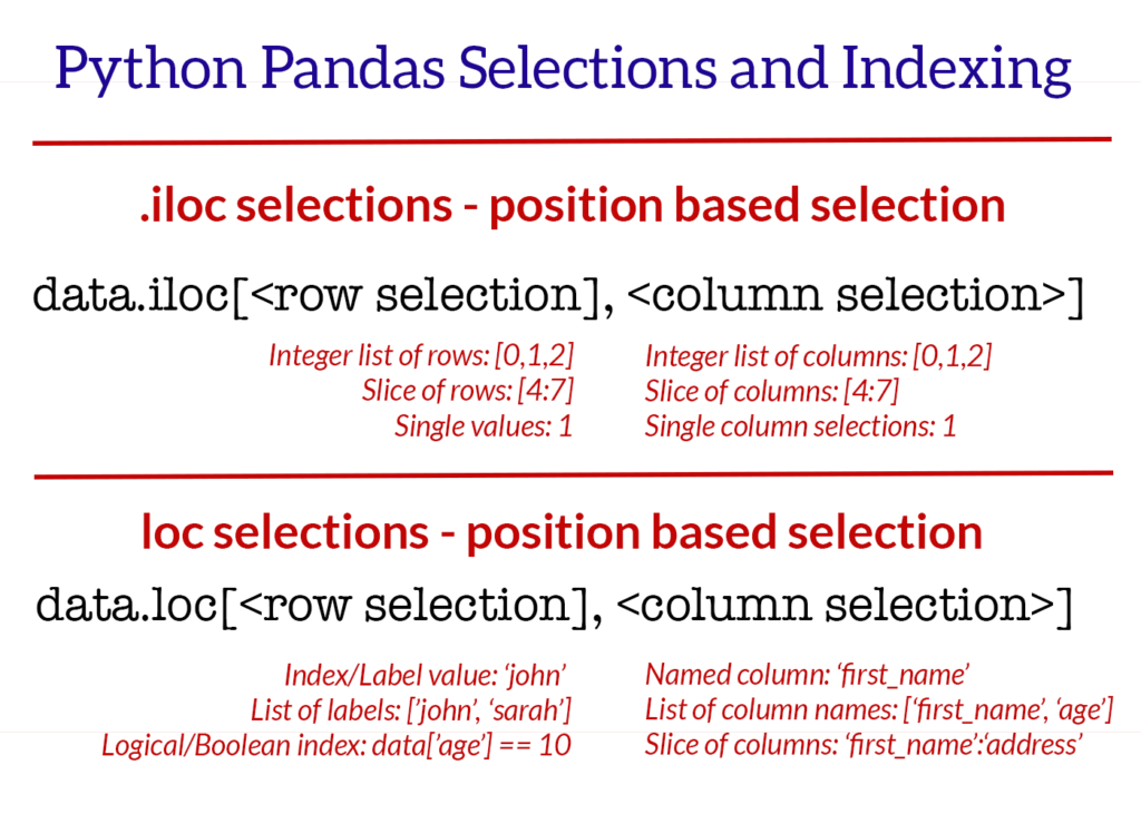
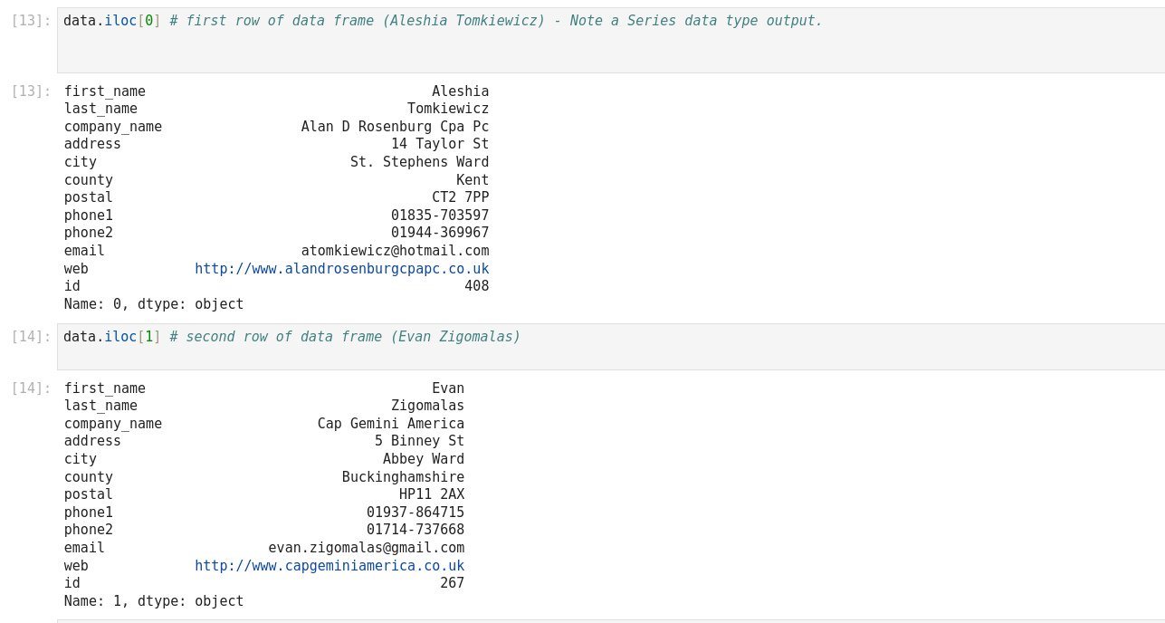
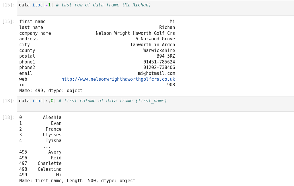
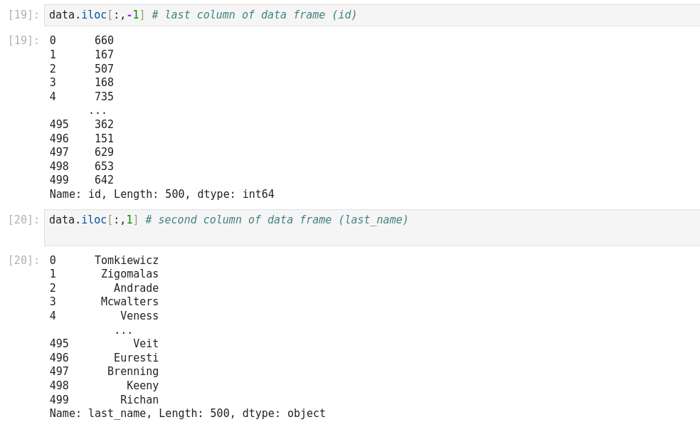
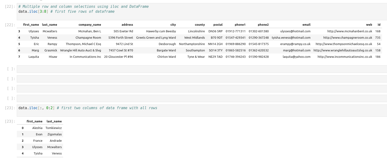
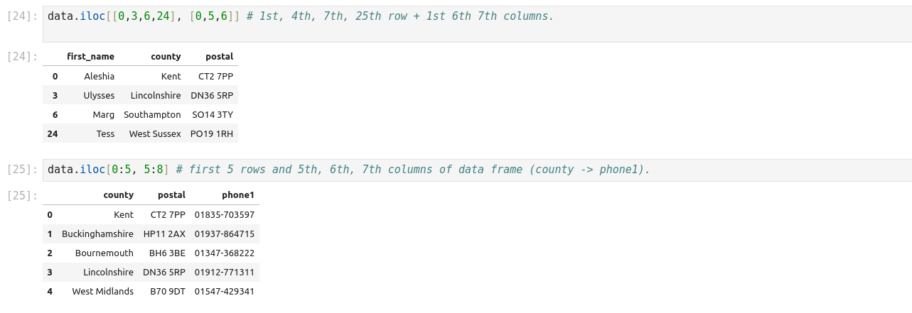
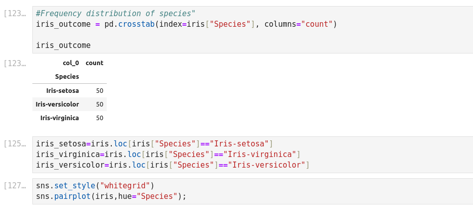
La fonction iloc dans Pandas est un outil puissant qui permet la manipulation et l’analyse des données. Il s’agit d’une technique fondamentale qui peut être utilisée pour filtrer, découper et sélectionner des données à partir d’un Pandas DataFrame. Iloc est une fonction Pandas qui signifie localisation entière. Il est utilisé pour sélectionner des lignes et des colonnes d’un DataFrame en fonction de leur position entière. Cela signifie qu’iloc vous permet de sélectionner des données en fonction de leur position dans un DataFrame, plutôt que de leur étiquette ou de leur valeur. Pour utiliser iloc, vous devez spécifier la position entière des lignes et des colonnes que vous souhaitez sélectionner. La syntaxe d’utilisation d’iloc est la suivante :

Df.iloc[row_index, column_index]

Iloc et loc sont toutes deux des fonctions Pandas utilisées pour sélectionner des données à partir d’un DataFrame, mais elles fonctionnent différemment. Iloc sélectionne les lignes et les colonnes en fonction de leur position entière, tandis que loc sélectionne les lignes et les colonnes en fonction de leur étiquette ou de leur valeur. En général, iloc est plus rapide que loc car il fonctionne sur des positions entières plutôt que sur des étiquettes.

Data Manipulation with Pandas (p. 197)

NOTES COMPLÉMENTAIRES SUR ILOC

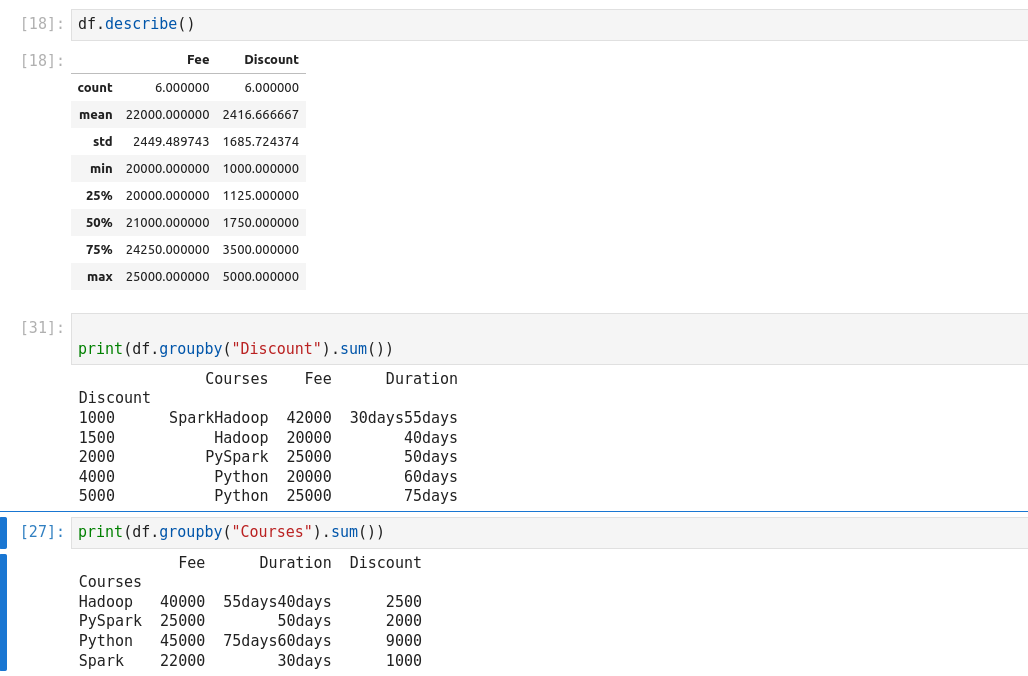
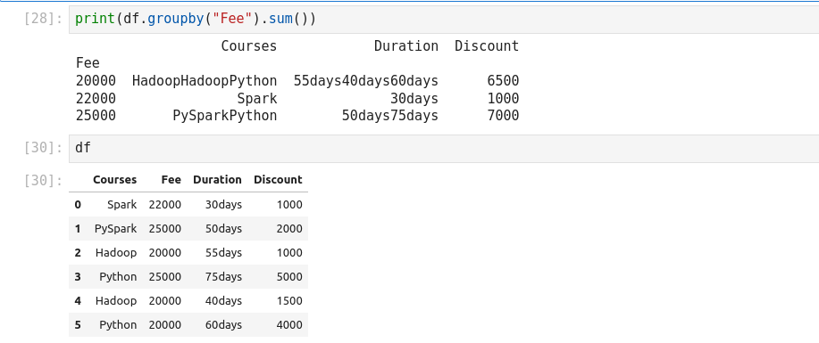
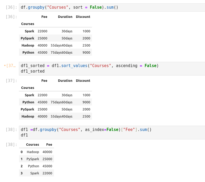
groupby essentially splits the data into different groups depending on a
variable of choice to perform computations for better analysis. Groups data on
Courses column and calculates the sum for all numeric columns of DataFrame.

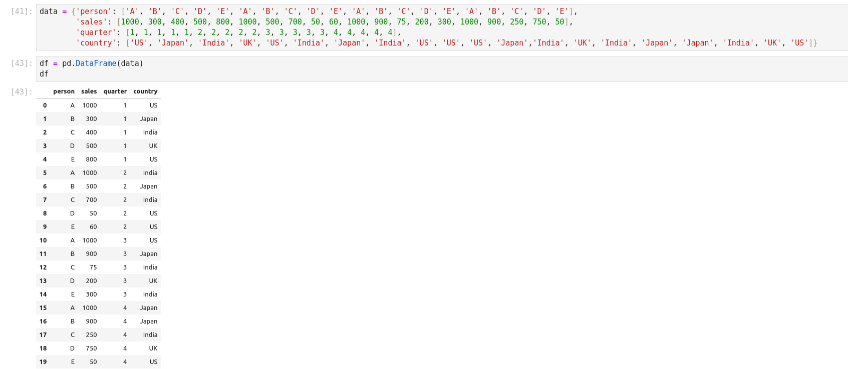
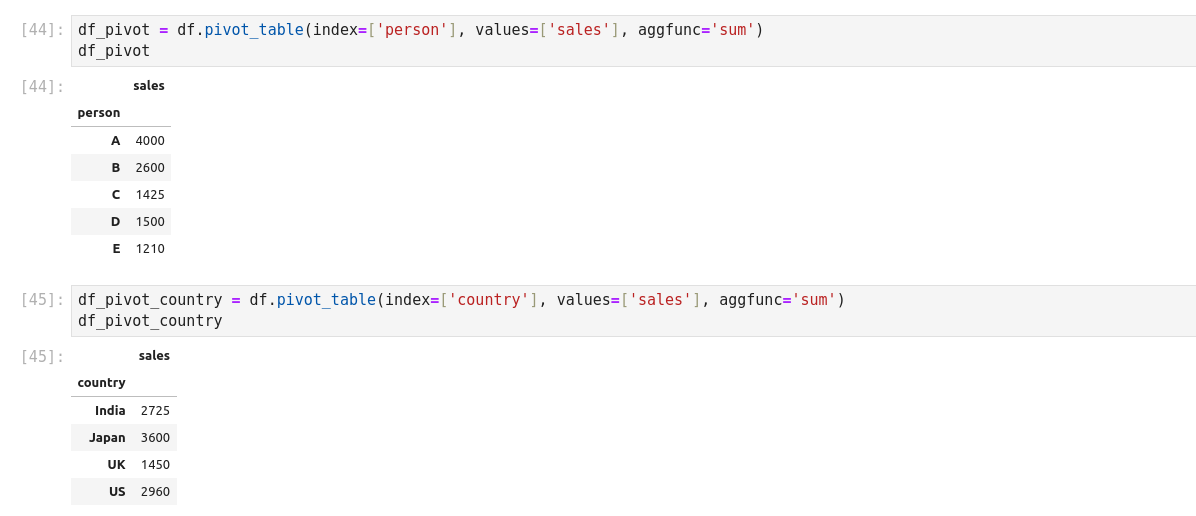
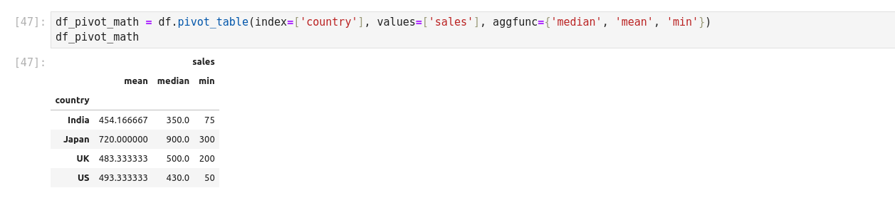
Pivot Tables

A pivot table is a similar operation that is commonly seen in spreadsheets and other programs that operate on the tabular data. The pivot table takes a simple column wise data as input, and groups the entries into two-dimensional table that provides a multidimensional summary of the data. Pivot tables are made possible through groupby facility combined with reshape operations utilizing hierarchical indexing. DataFrame has a pivot_table method.

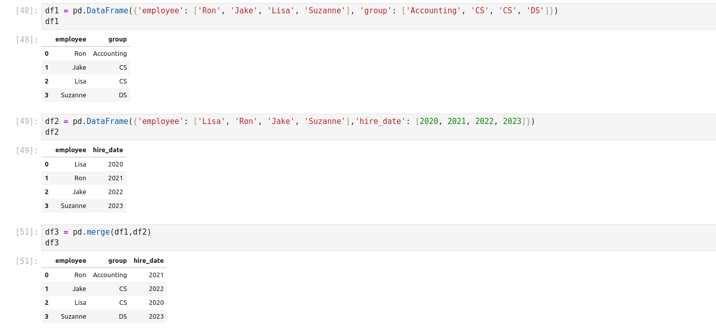
Merge 2 pivot table:

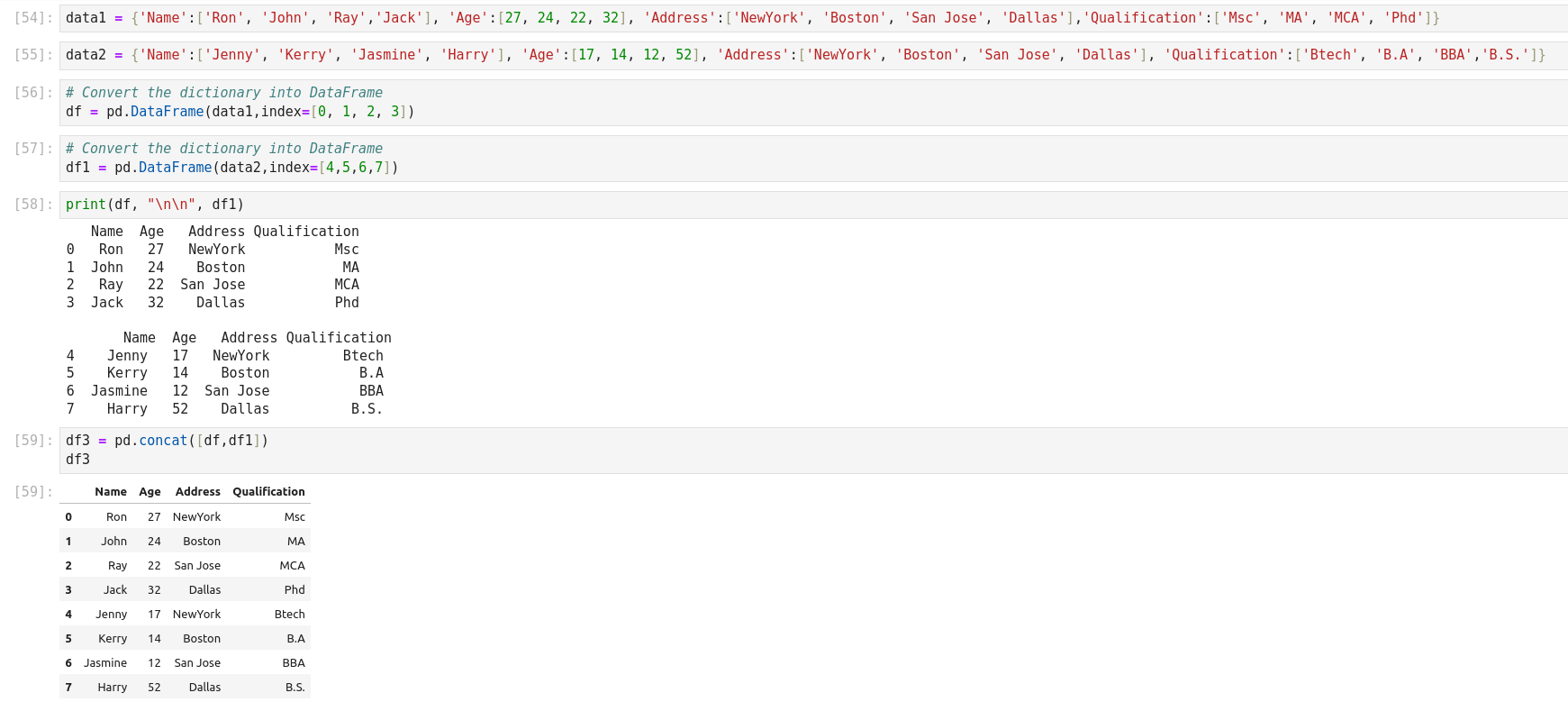
Concatenation of Series and DataFrame objects is very similar to concatenation of NumPy arrays.

Concatenating DataFrame using pd.concat()
Concatenating DatafRames by setting logic or axes
Concatenating DatafFrame using .append()
Concatenating DataFrame by ignoring indexes
Concatnating DataFrame with group keys
Concatenating with mixd ndimd

Data Cleaning

Standardizing data
Identifying and fixing errors
Removing incorrect data
Correcting format
Checking the accuracy of information
Compiling all data information in a single data

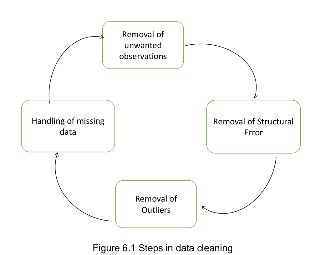
Data cleaning is the process that removes data that does not belong in dataset. Data transformation is the process of converting data from one format or structure into another. tfrom one “raw” data form into another format for warehousing and analyzing.

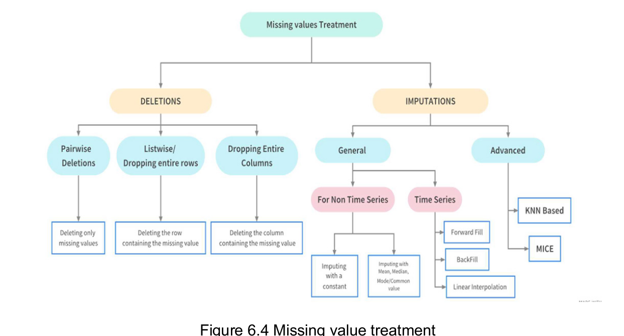
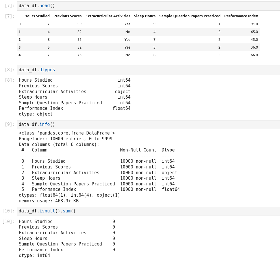
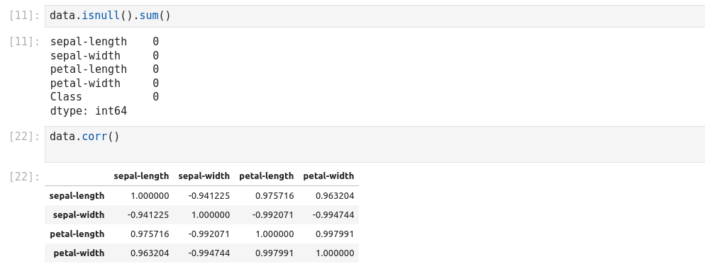
There are several useful methods for detecting, removing, and replacing null values in Pandas data structure. They are:
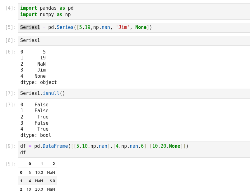
- isnull(): Generate a boolean mask indicating missing values
- notnull(): Opposite of isnull()
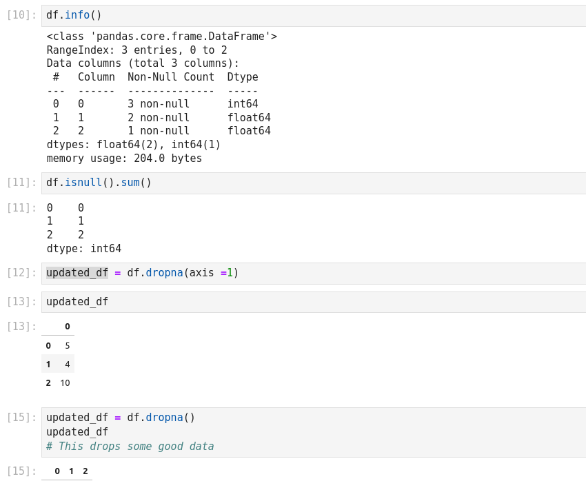
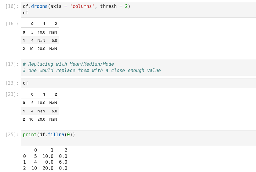
- dropna: Return a filtered version of the data
- fillna(): Return a copy of the data with missing values filled or imputed.

There are the conventional methods, such as dropna() (which removes NA values) and fillna() (which fills in NA values).

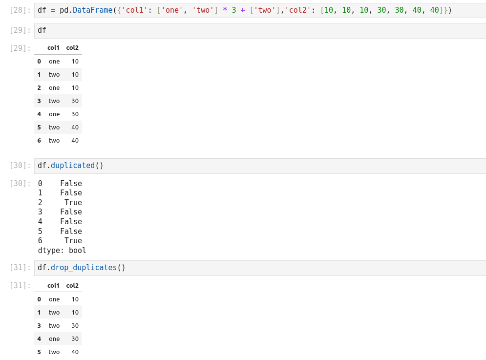
Valeurs dupliquées:

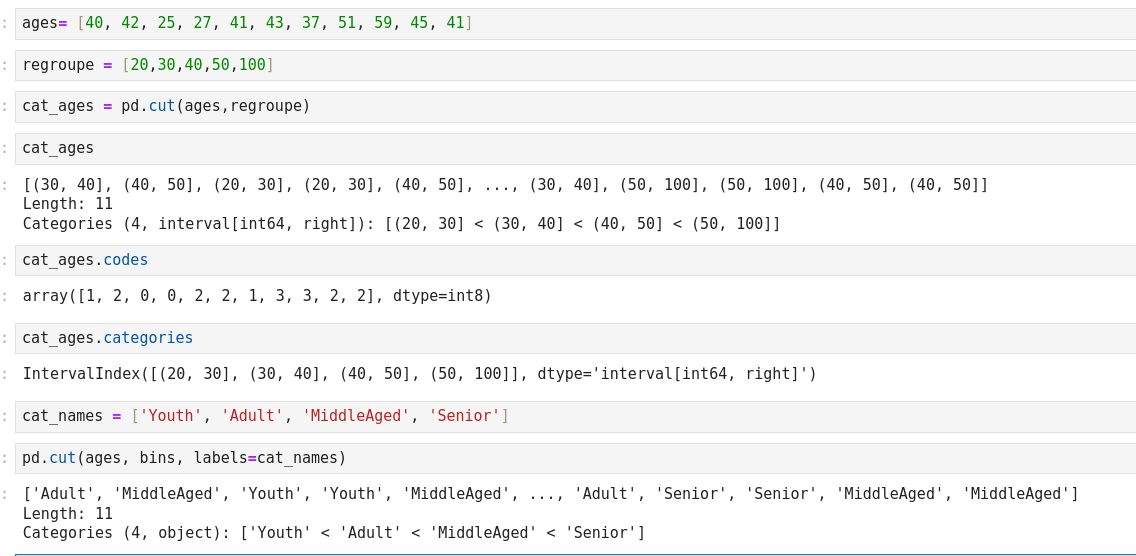
Discretization and Binning (regroupement)

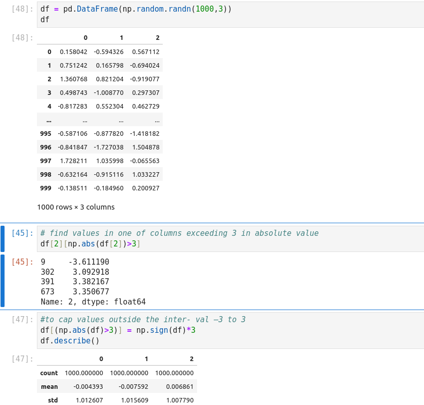
Detecting Outliers

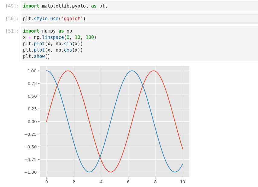
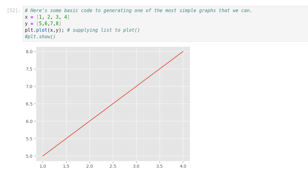
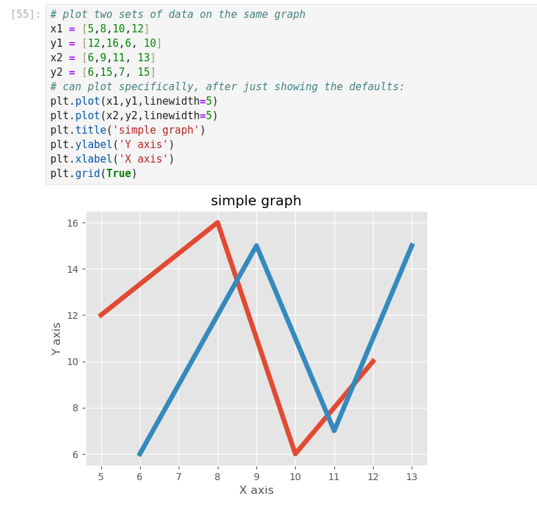
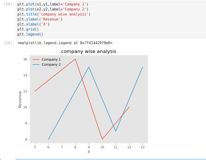
Data Visualization with Python

Fast and easy decision making
More people involved
Higher degree of involvement
Better understanding
Keep Audience in Mind
Determine the best visual
Balance the design
Focus on the key areas
Keep in simple
Use patterns
Compare aspects
Showing change over time
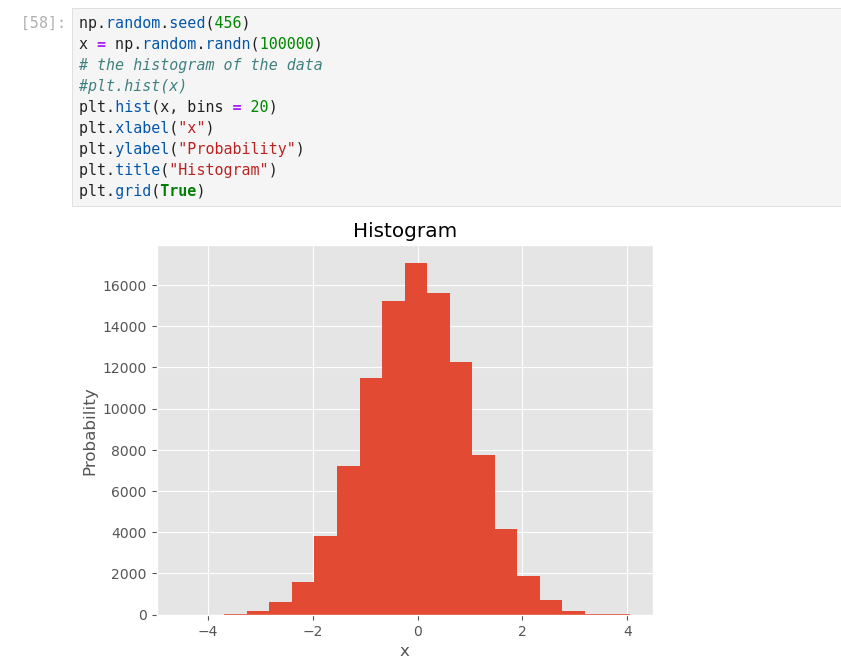
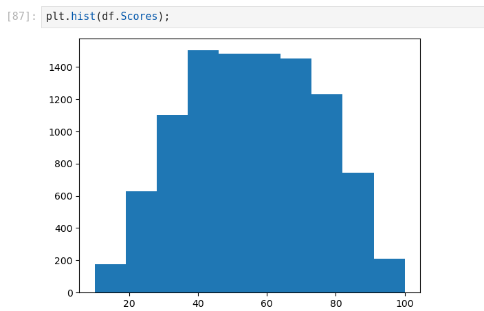
Looking at how data is distributed
Comparing values between groups
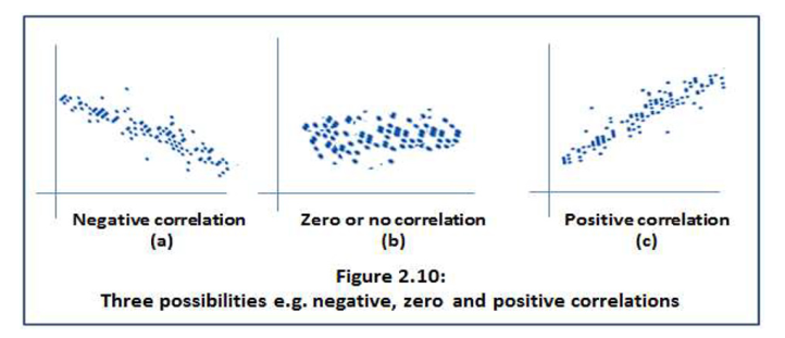
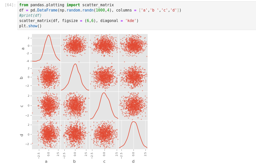
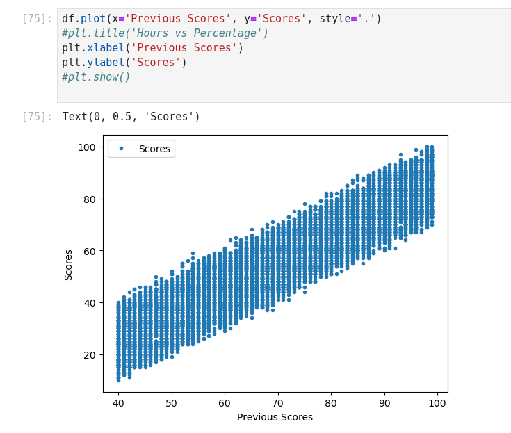
Observing relationships between variables
Looking at geographical data

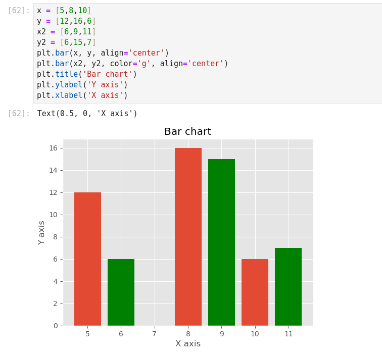
Bar charts
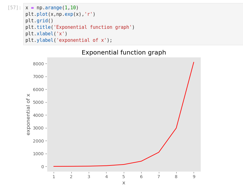
Line charts
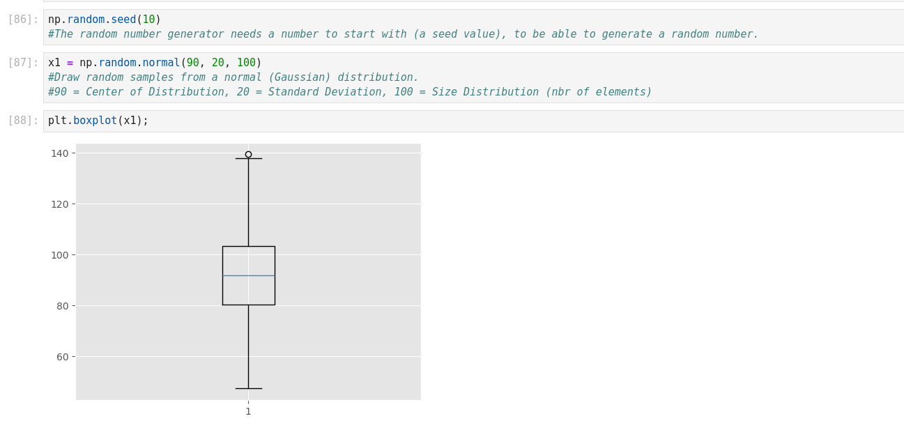
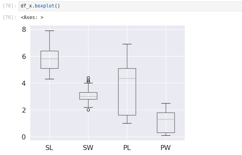
Box plot
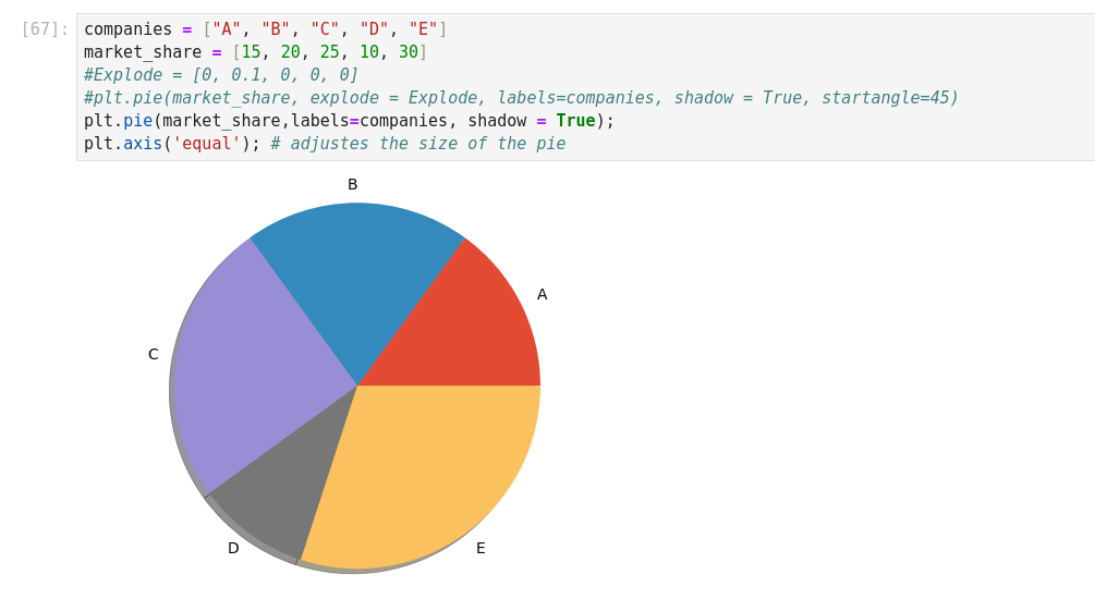
Pie chart
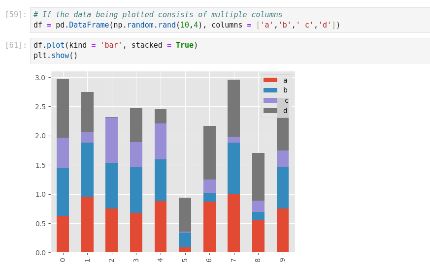
Stacked bar chart
Stacked area chart
Violin plot

Visualization packages

Matplotlib
Seaborn
Plotly
Bokeh
Folium
ggplot
Geoplotlib
Missingno

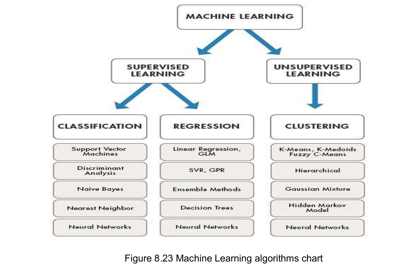
Machine Learning

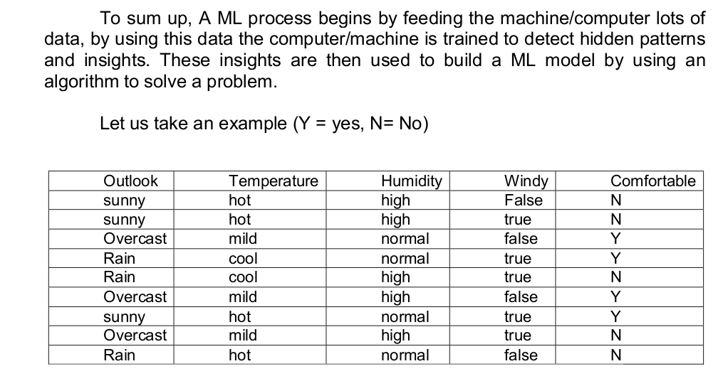
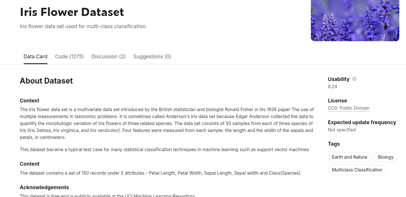
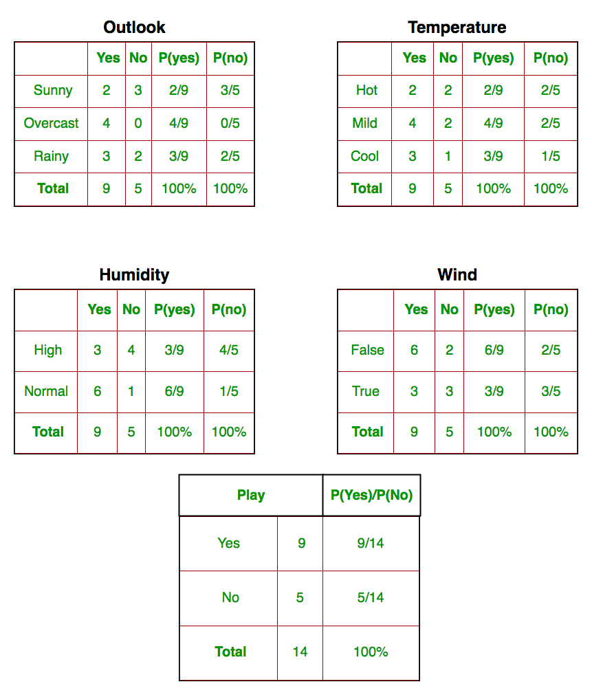
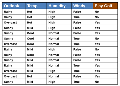
In the above example there are five features (Outlook, Temperature, Humidity, Windy, and Comfortable). There are 9 observations. In this example Class is the target (play or no play) that ML algorithm wants to learn and predict for unseen new data. This is a typical classification problem.

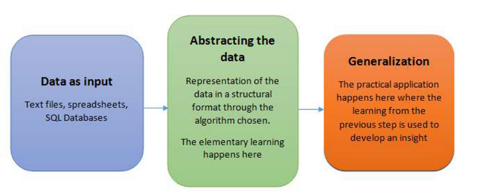
How do machines learn?

Steps to Apply ML

Problem definition
Data Collection/Data Extraction
Prepare the data
Train the algorithm
Test the algorithm
Improving the performance
Deployment

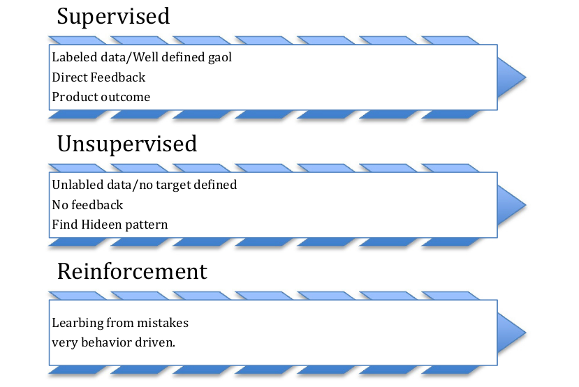
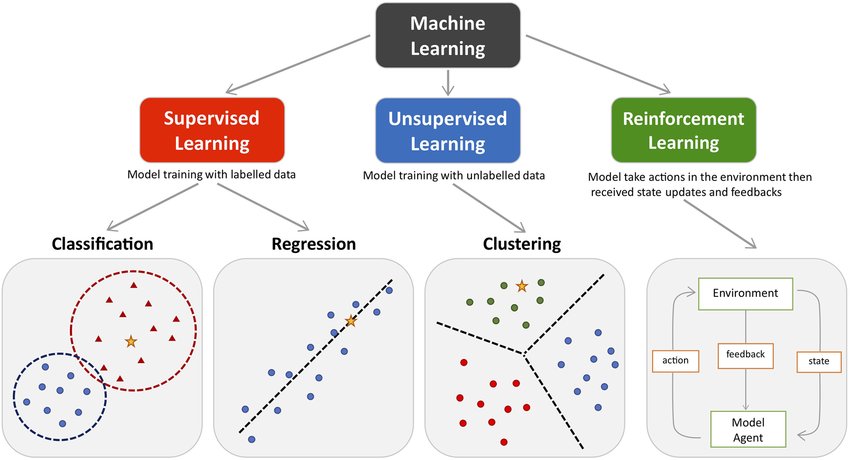
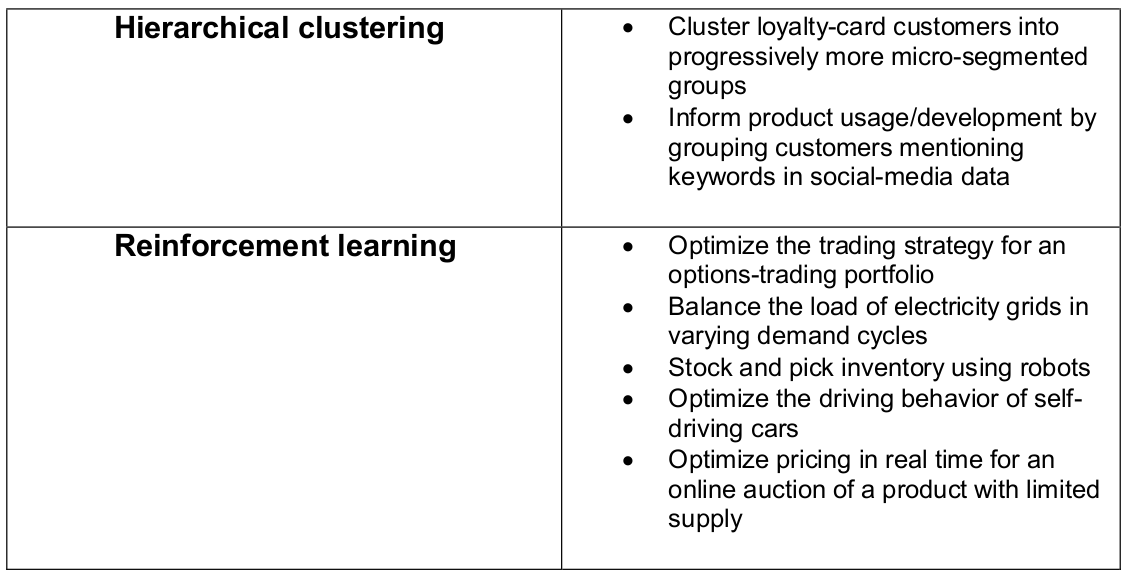
Paradigms of Learning

There is No Free Lunch Theorem famous in Machine Learning. It states that there is no single algorithm that will work well for all the problems. Each problem has its own characteristics/properties. There
are basic three types of learning paradigms:

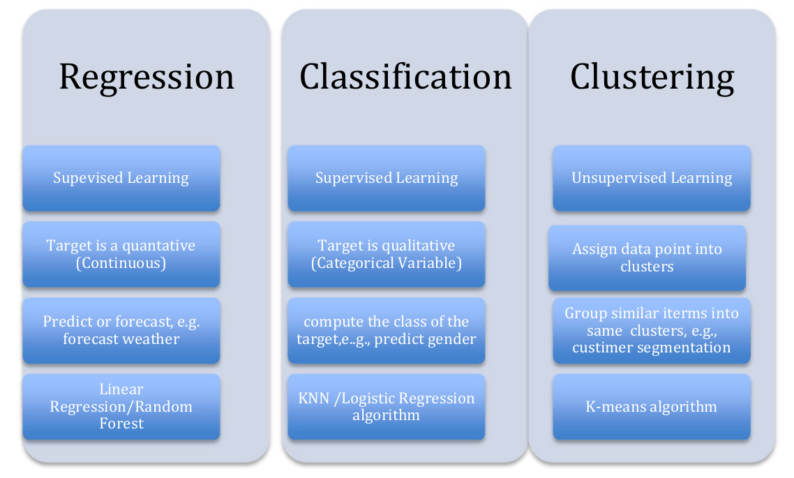
Type of Problems in Machine Learning

Machine Learning/Artificial Intelligence is everywhere

Virtual personal assistants
Predictions while commuting
Video surveillance
Social media services
Email Spam and Malware Filtering
Product recommendation, online fraud detection

Computing Requirements

If tasks are small and can fit in a complex sequential processing, one does not need a big system. One can even skip the GPUs altogether. A CPU such as i7-7500U can train an average of ~115 examples/second. So if you are planning to work on other ML areas or algorithms, a GPU is not necessary.

If task is computing intensive, and has manageable data, a reasonably powerful GPU would be a better choice. A laptop with a dedicated graphics card of high end should suffice. There are a few high end (and expectedly heavy duty) laptops like Nvidia GTX 1080 (8 GB VRAM), which can train an average of ~14k
examples/second for a mid-size problem. In addition, you can build your own PC with a reasonable CPU and a powerful GPU, but bear in mind that the CPU must not bottleneck the GPU. For instance, an i7-7500U will work flawlessly with a GTX 1080 GPU.

GPU: This is the most important aspect as Deep Learning, which is a Sub-Field of Machine Learning requires neural networks to work and are computationally expensive. Working with Images or Videos requires heavy Matrix Computations. GPUs enable parallel processing of computations. Without GPU the process might take unacceptable amount of time.

Storage: A minimum of 1TB HDD is required as the datasets tend to get larger and larger by the day. With a system having SSD a minimum of 256 GB is advised. Then again if one may have less storage one can opt for Cloud Storage Options. Cloud can provide machines with high GPUs even.

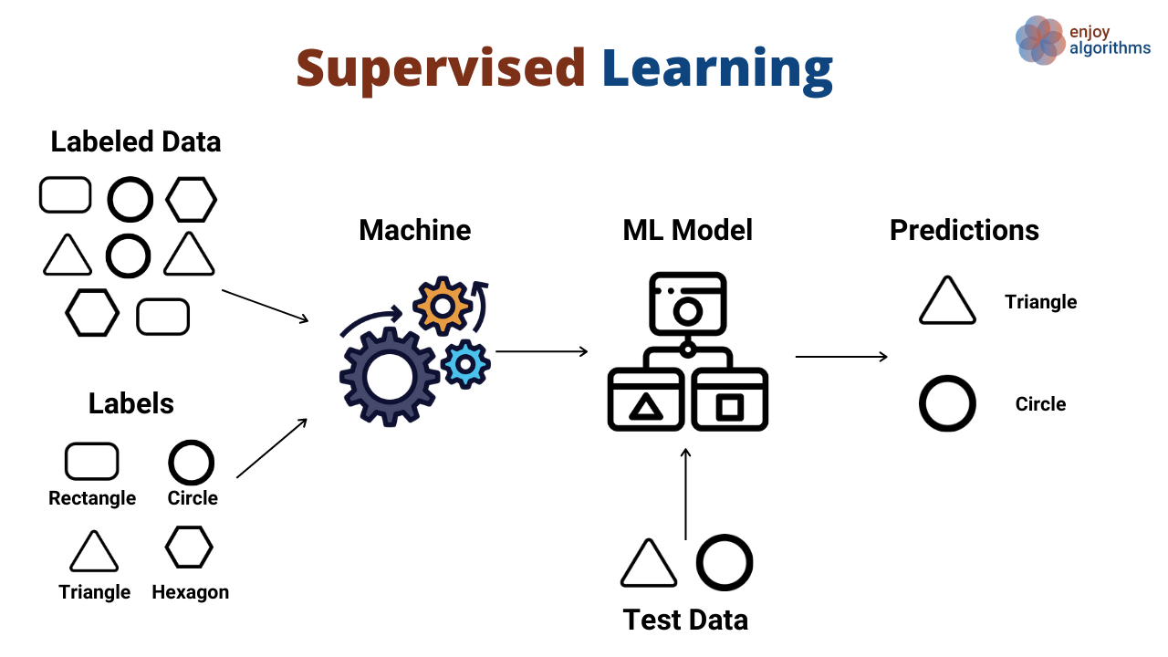
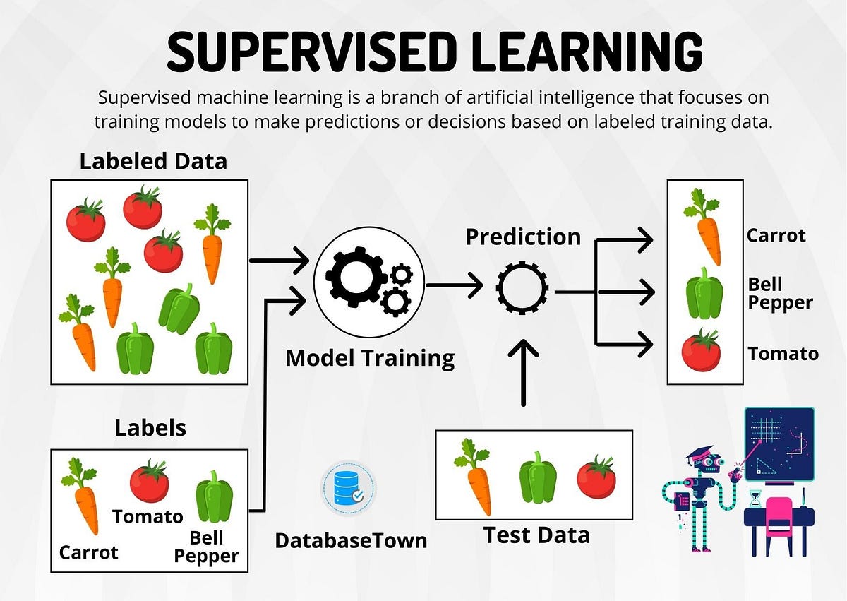
Supervised Machine Learning Algorithms

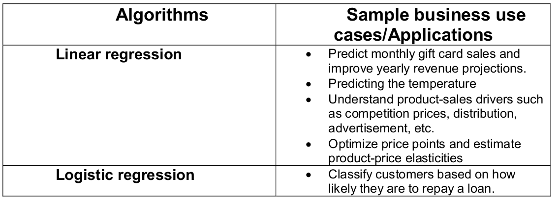
Popular machine learning algorithms

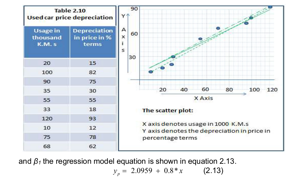
Linear Regression
Logistic Regression
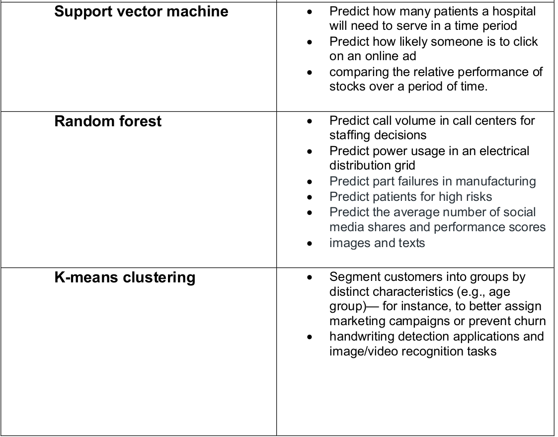
Support Vector Machines
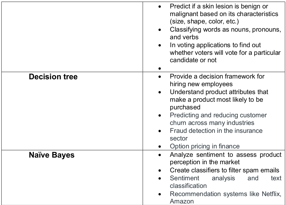
Naive Bayes
Decision Trees
Random Forest
Artificial Neural Networks
K-Nearest Neighbors (KNN)

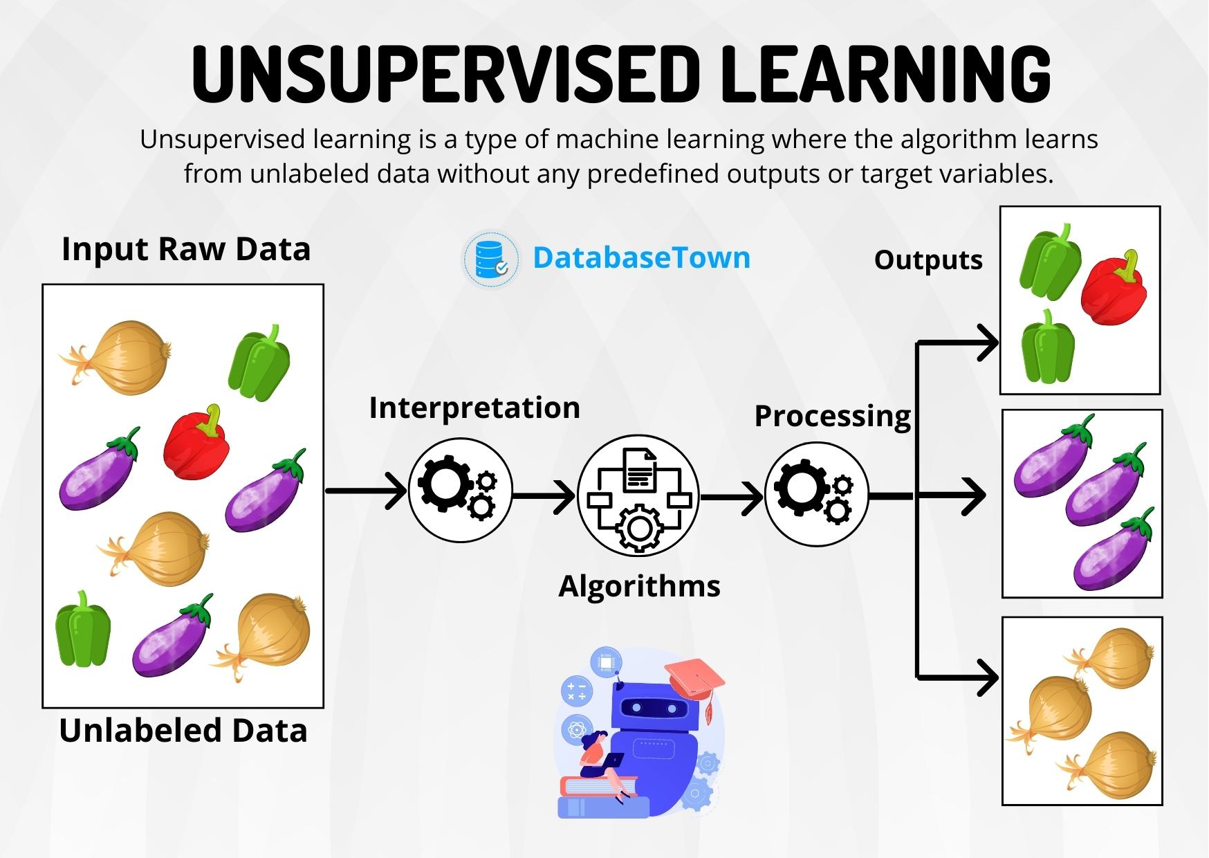
Unsupervised Machine Learning Algorithms

This method does not involve training the model based on old data.

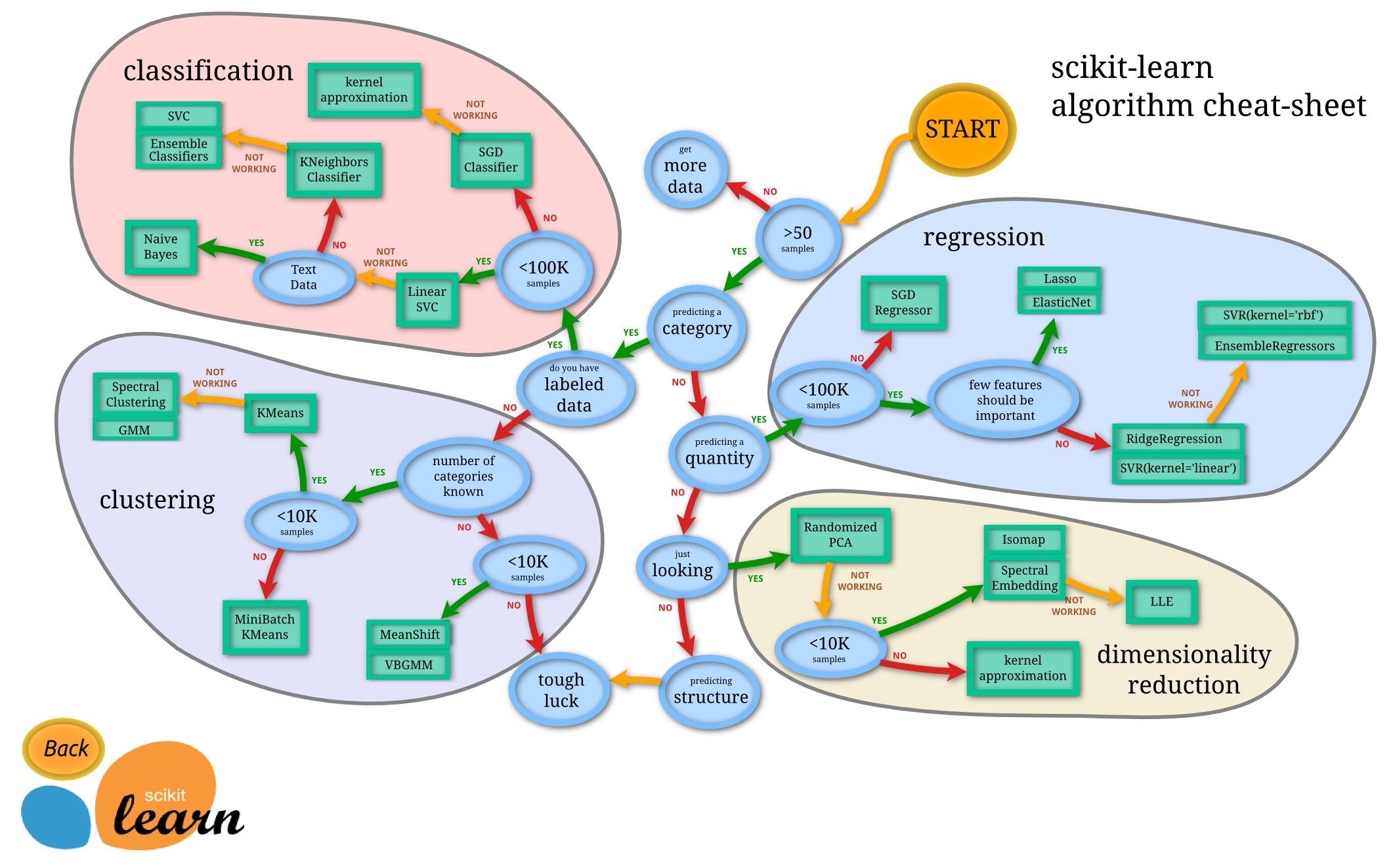
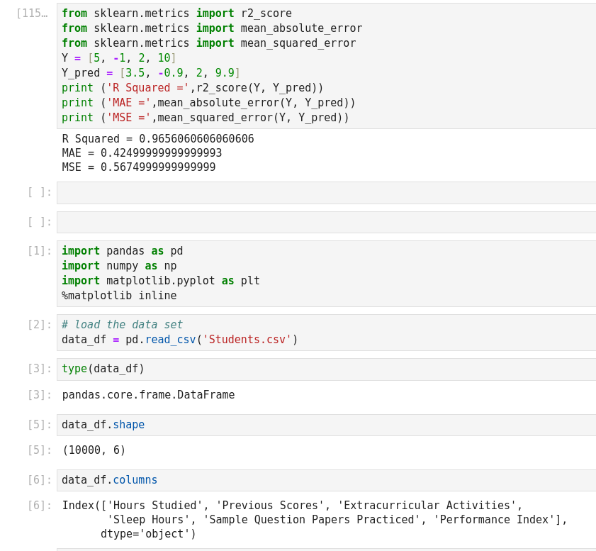
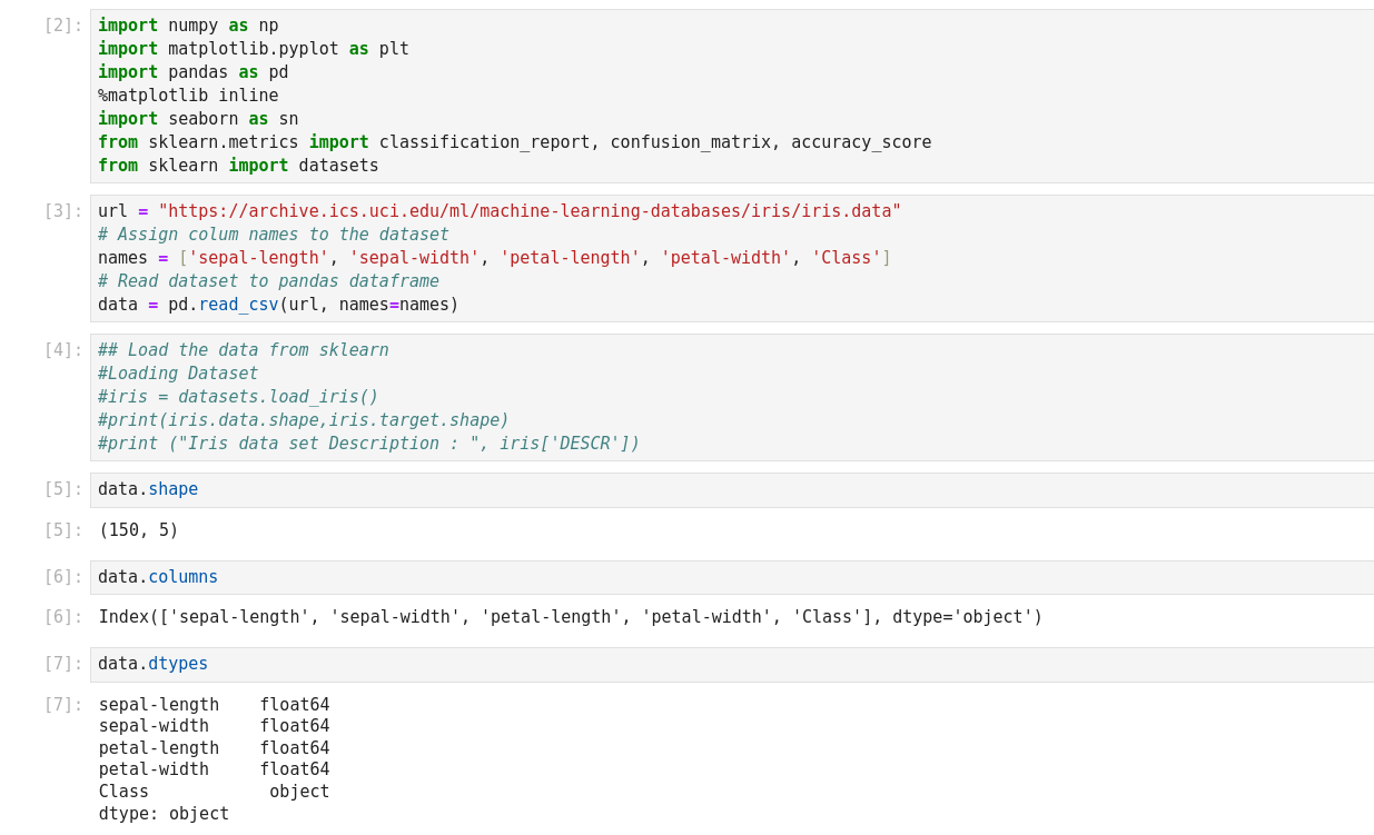
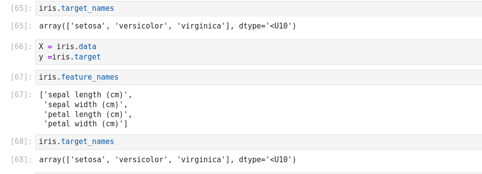
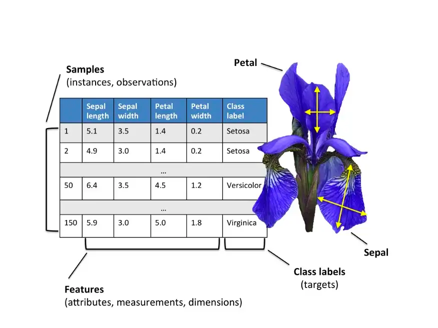
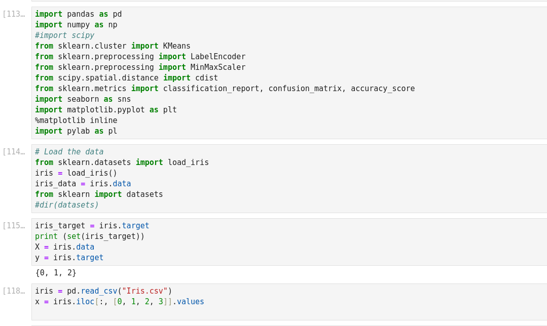
Scikit-Learn

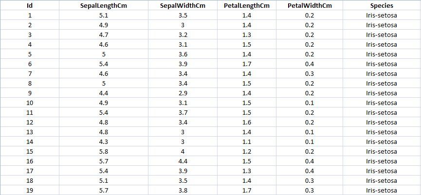
Importing the dataset. One can load the dataset with Pandas.
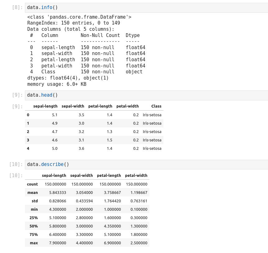
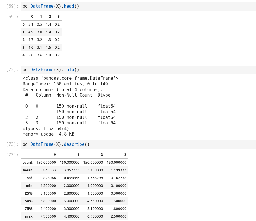
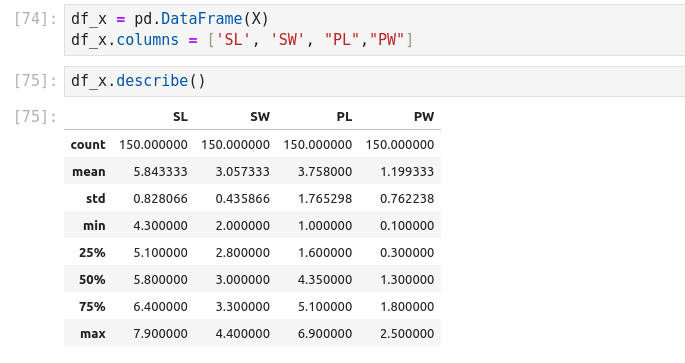
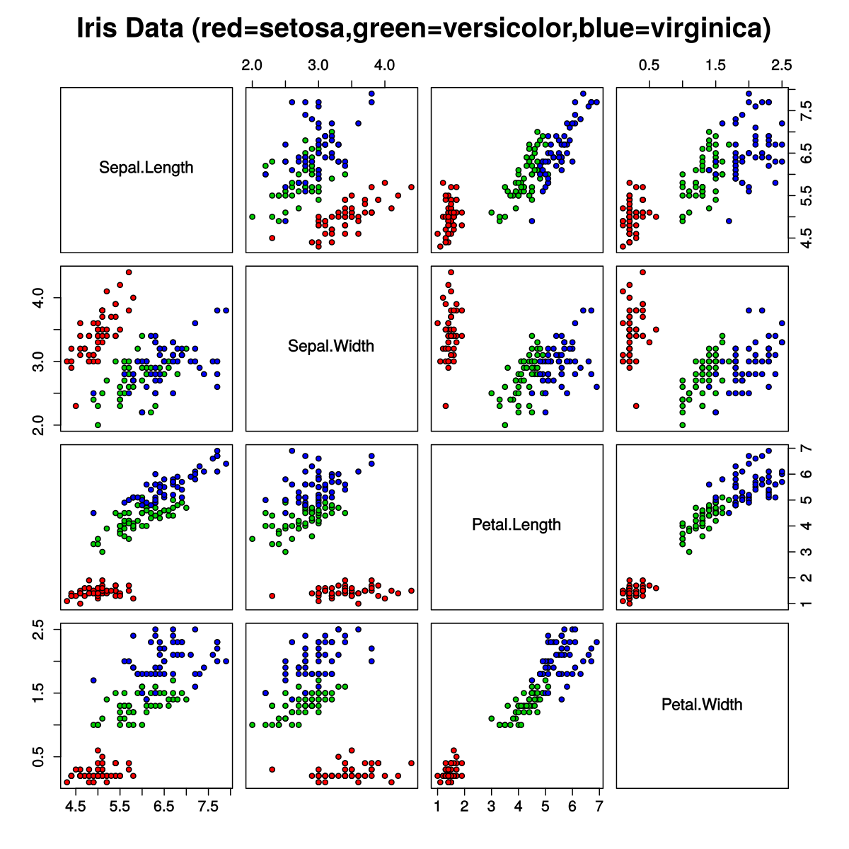
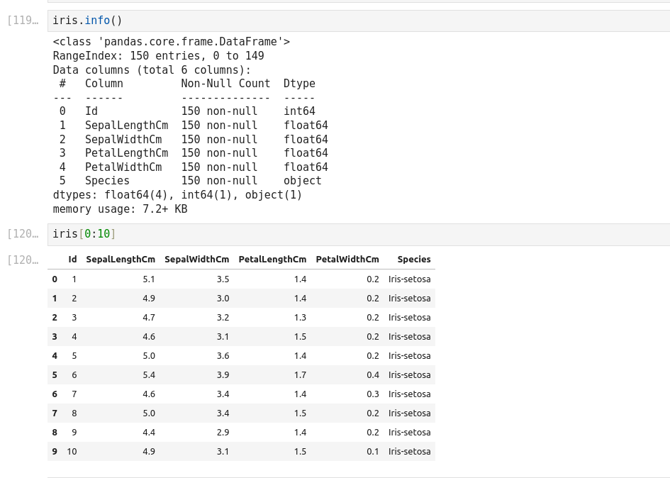
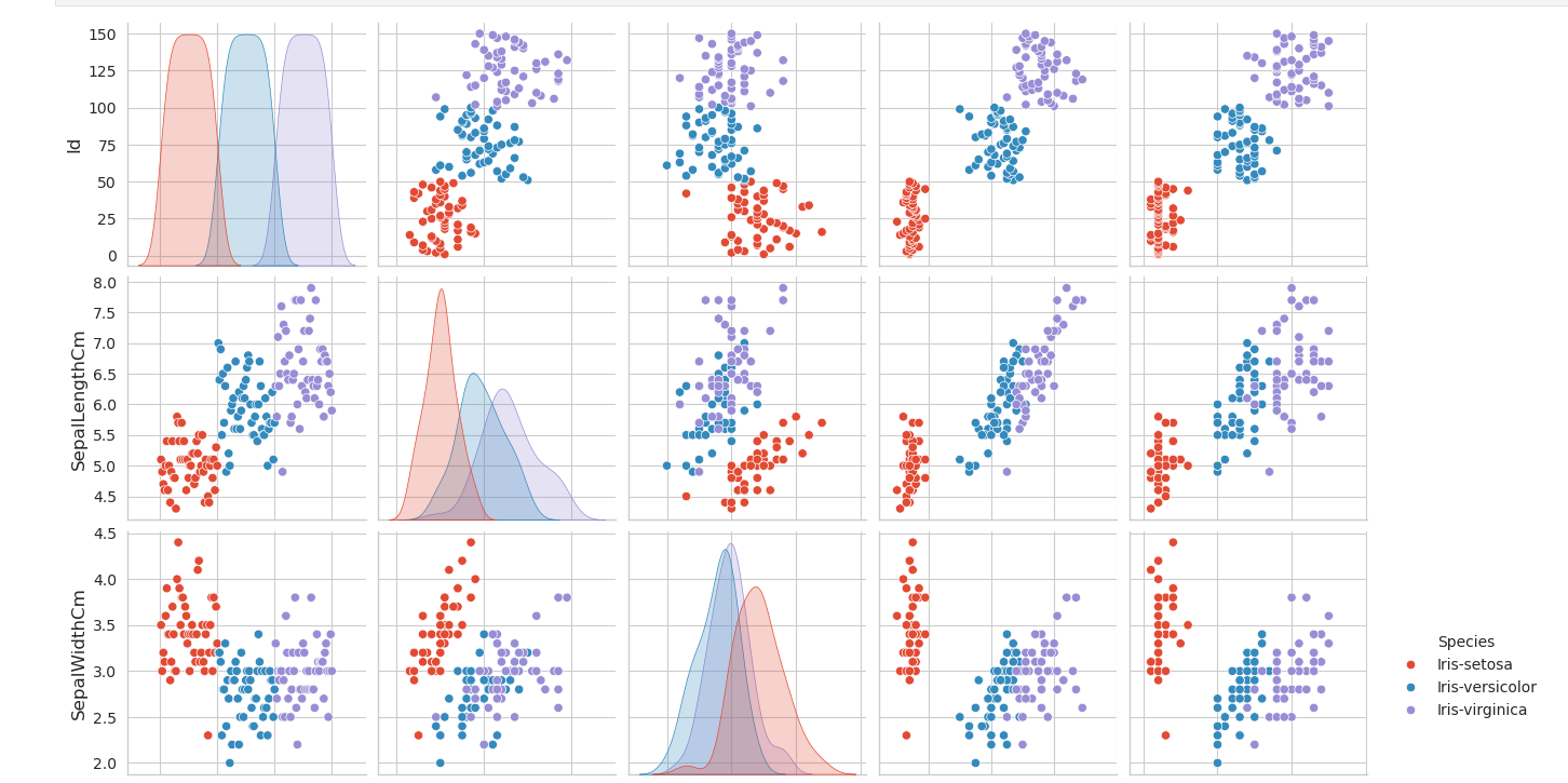
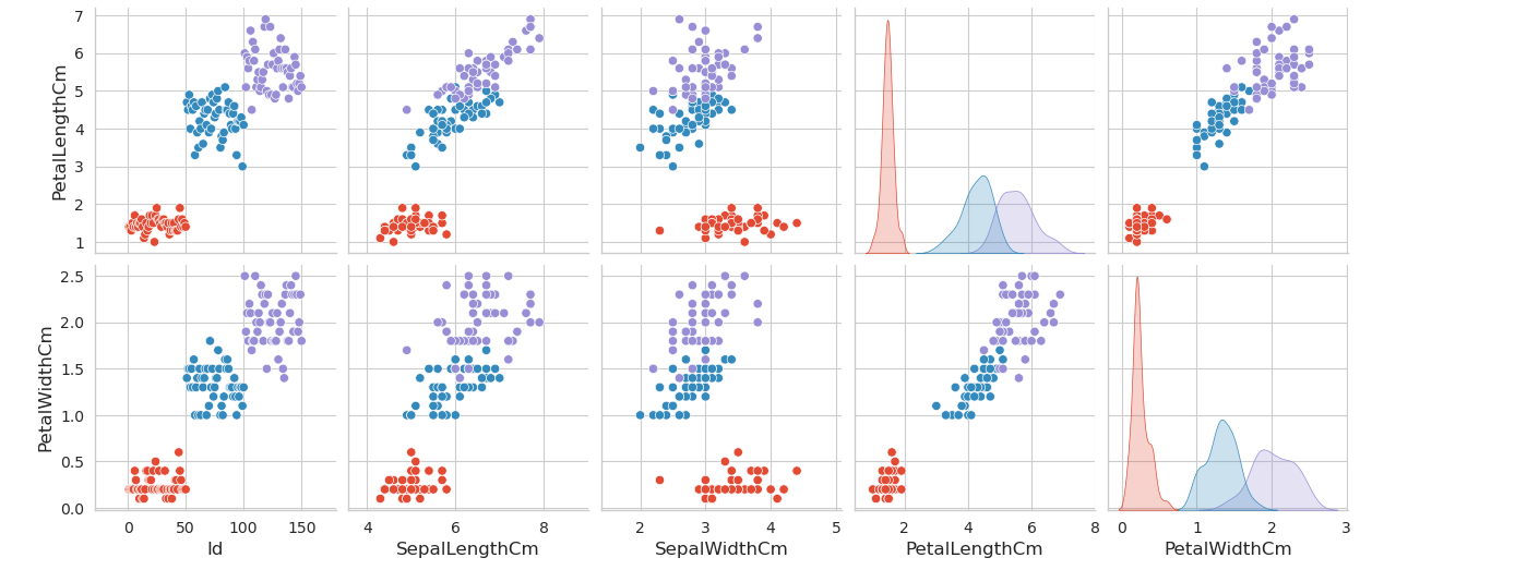
Exploring the data
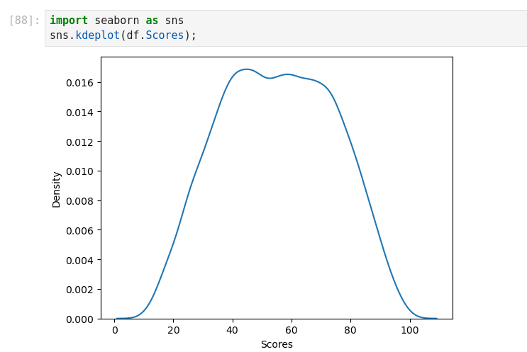
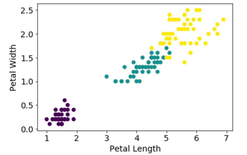
Data Visualization
Preparing the data
Selecting features
Training and testing (learning and predicting)

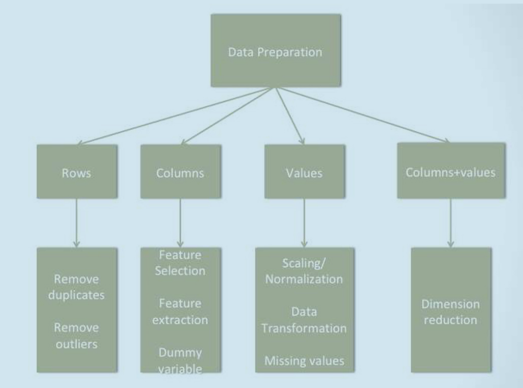
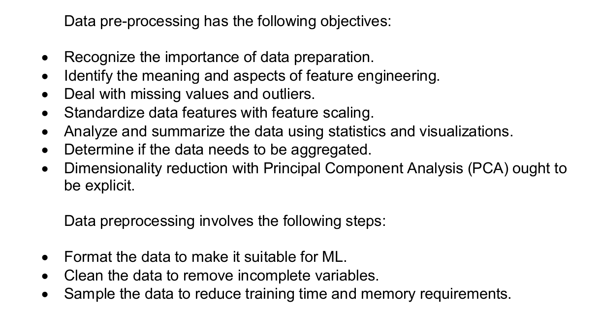
Data Preparation: transforming raw data into meaningful features for a data mining task
Data Selection (feature selection): some of these features can be irrelevant or redundant, and may negatively influence the performance of the training activity.
Data Cleaning: the process of identifying and correcting (or removing) incomplete, improper, and inaccurate data.
Insufficient data: Selecting the right size of sample is a key step in data preparation.
Non-representative Data: The sample selected should be a fair representation of the entire data.
Substandard Data: Outliers, errors, and noise can be eliminated to get a better fit of the model.
Data Transformation: Scaling & Aggregation

Handling Missing Values
- Deleting Rows
- Replacing With Mean/Median/Mode
- Assigning A Unique Category
- Predicting The Missing Values

Performance Metrics of ML Algorithms

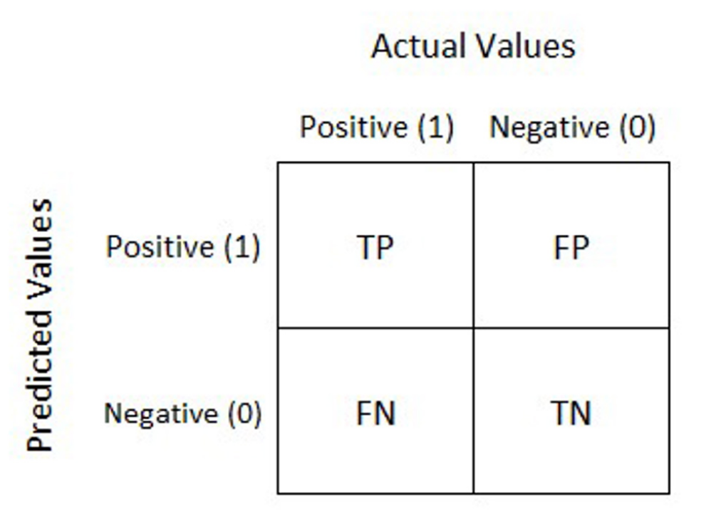
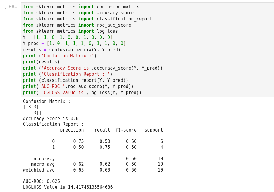
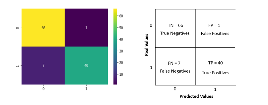
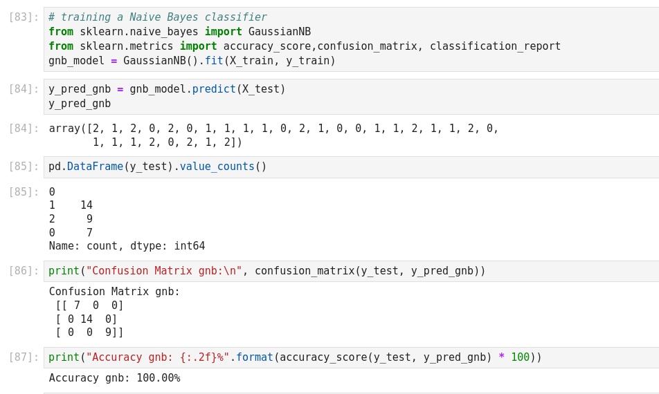
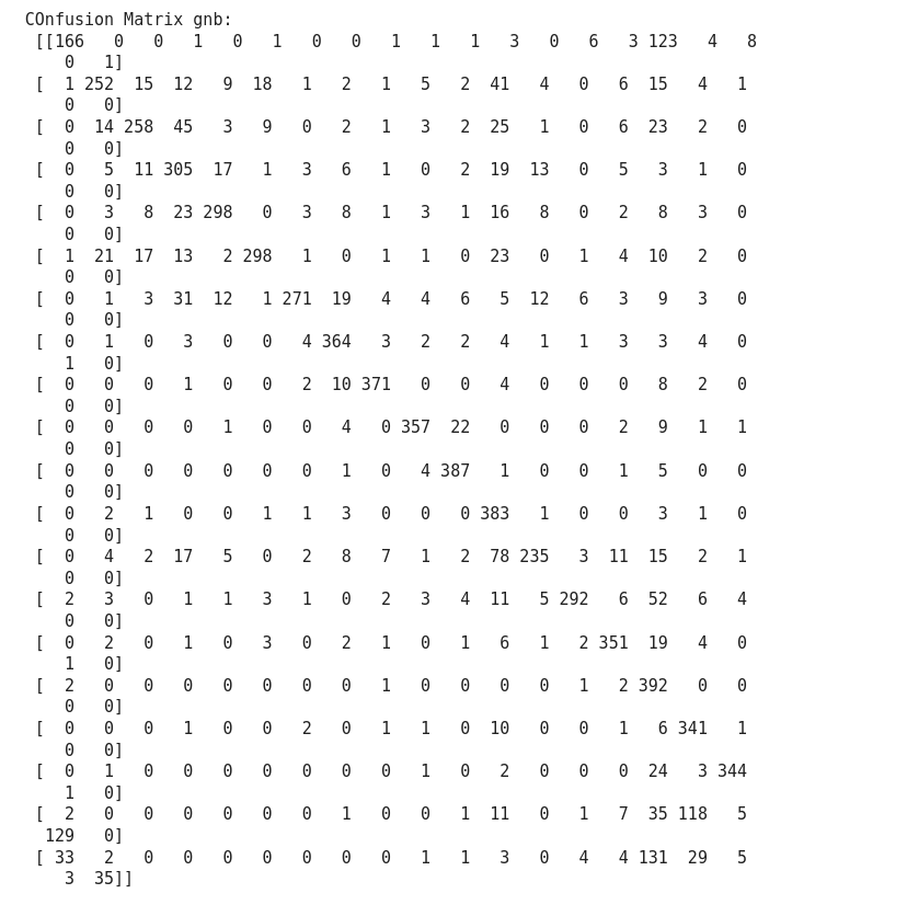
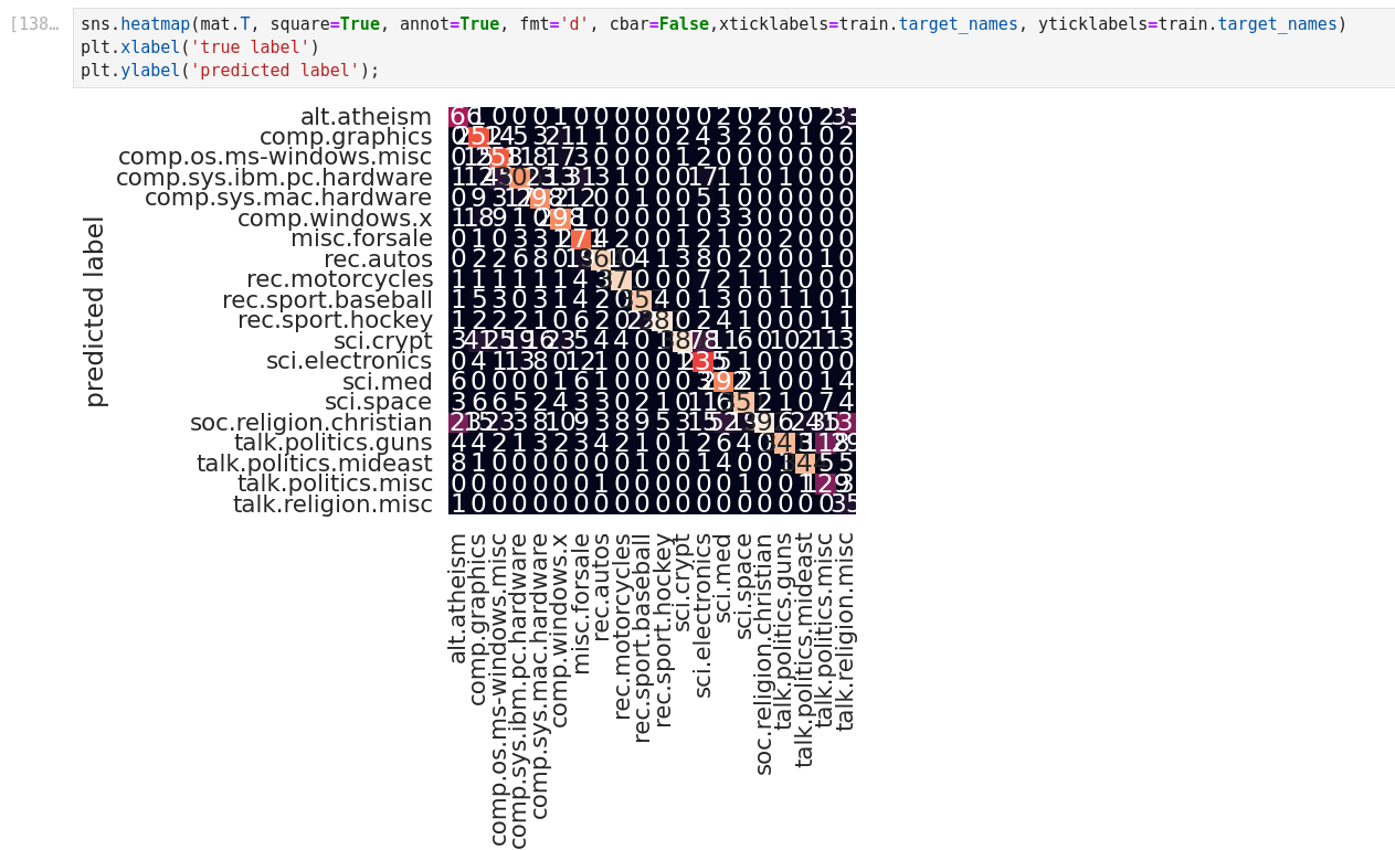
Confusion matrix: Confusion matrix gives us a matrix output and describes the complete performance of the model.

True Positives (TP): It is the case when both actual class and predicted class of data point is 1.
True Negatives (TN): It is the case when both actual class and predicted class of data point is 0
False Positives (FP): It is the case when actual class is 0 and predicted class of data point is 1. It is also known as Type I error.
False Negatives (FN): It is the case when both actual class is 1 and predicted class of data point is 0. It is also known as Type II error.

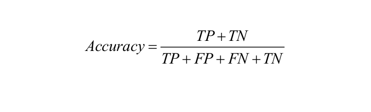
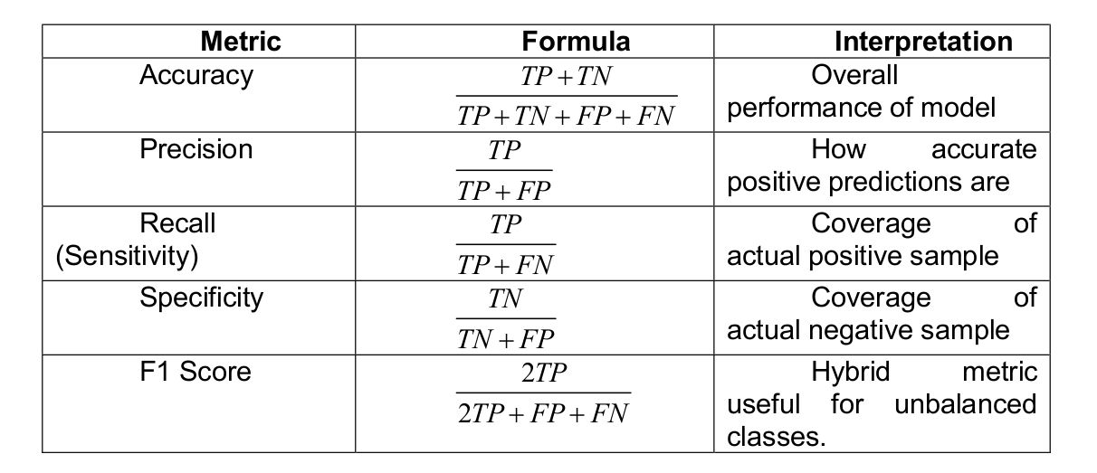
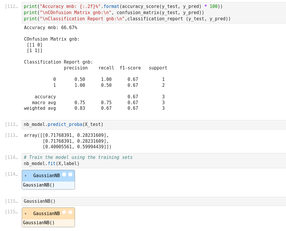
Accuracy: It is defined as the number of correct predictions made as a ratio of all the predictions made.

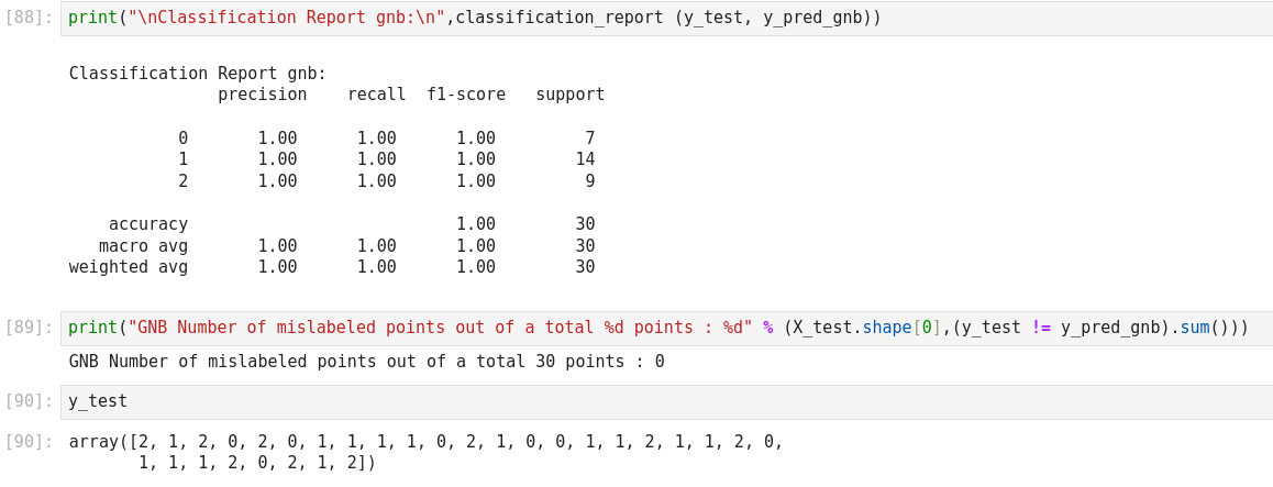
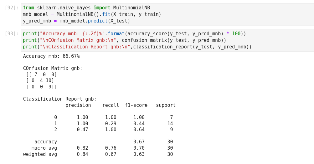
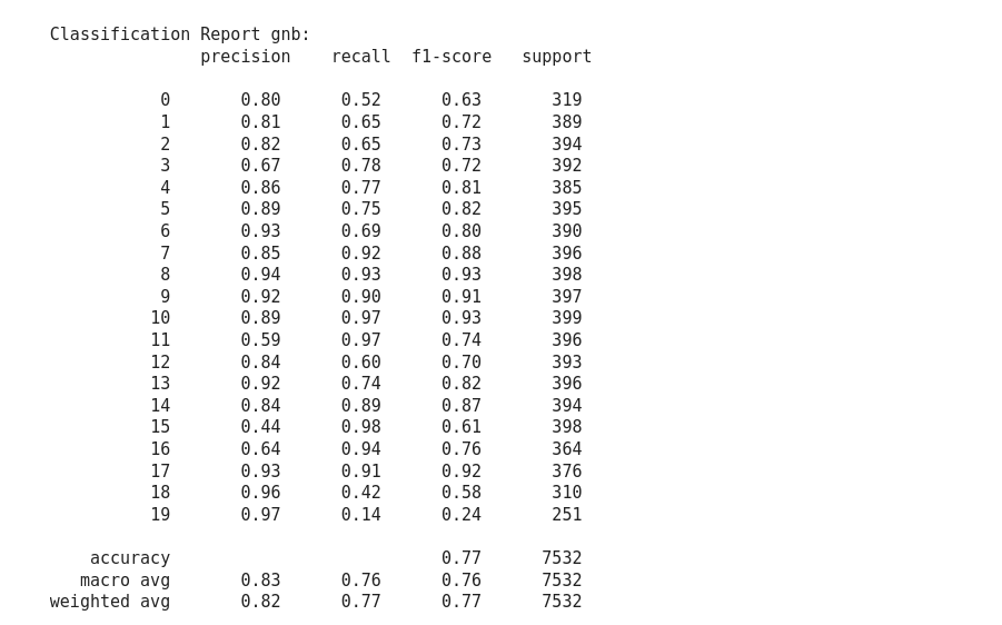
Classification Report: This report consists of the scores of Precisions, Recall, F1 and Support.

Precision: It is the number of correct positive results divided by the number of positive results predicted by the classifier.

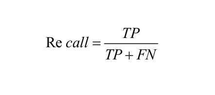
Recall or Sensitivity: It is the number of correct positive results divided by the number of all relevant samples

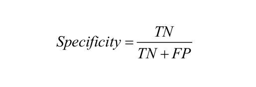
Specificity: Specificity is defined as the number of negatives returned by our ML model

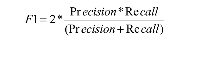
F1 Score: Mathematically, the range for F1 score is [0-1]. It tells how precise classifier is (how many instances it classifies correctly), as well as how robust it is (it does not miss significant number of instances). High precision but lower recall, gives an extremely accurate prediction, but then it misses a large number of instances that are difficult to classify. The greater the F1 score, the better is the performance of the model. F1 score tries to find a balance between precision and recall.

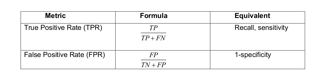
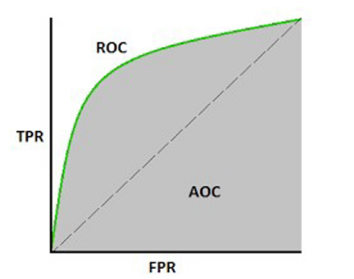
Receiver Operating Curve (ROC): ROC is the plot of True Positive Rate Versus False Positive Rate by varying the threshold.

Area Under ROC Curve (AUC)- The area under the ROC also known as AUC, is the area under the ROC

Mathematically, it can be created by plotting TPR (True Positive Rate) i.e., Sensitivity or recall vs FPR (False Positive Rate) i.e., 1-Specificity, at various threshold values. Following is the graph showing ROC, AUC having TPR at y-axis and FPR at x-axis

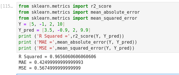
Regression metrics

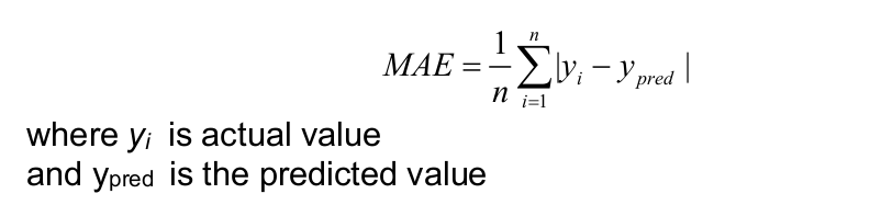
Mean Absolute Error (MAE): It is the sum of average of the absolute difference between the predicted and actual values.

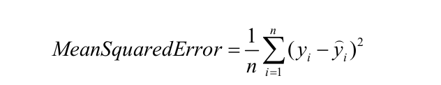
Mean Squared Error: Mean Squared Error (MSE) is quite similar to Mean Absolute Error, the only difference being that MSE takes the average of the square of the difference between the original values and the predicted values.

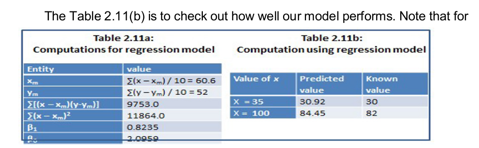
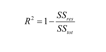
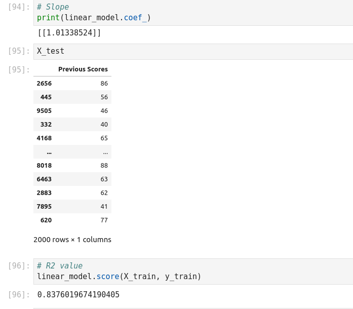
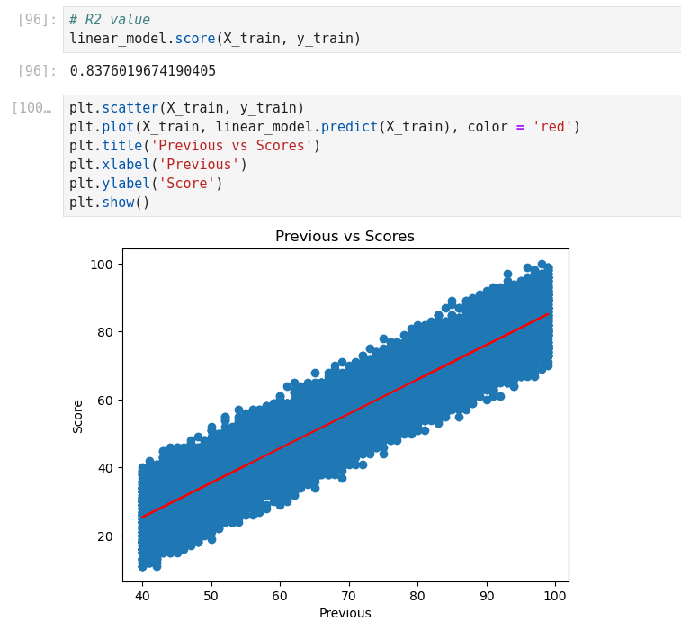
Coefficient of determination: R squared metric is generally used for explanatory purpose and provides an indication of the goodness of fit of predicted values to the actual output values,

Popular ML algorithms

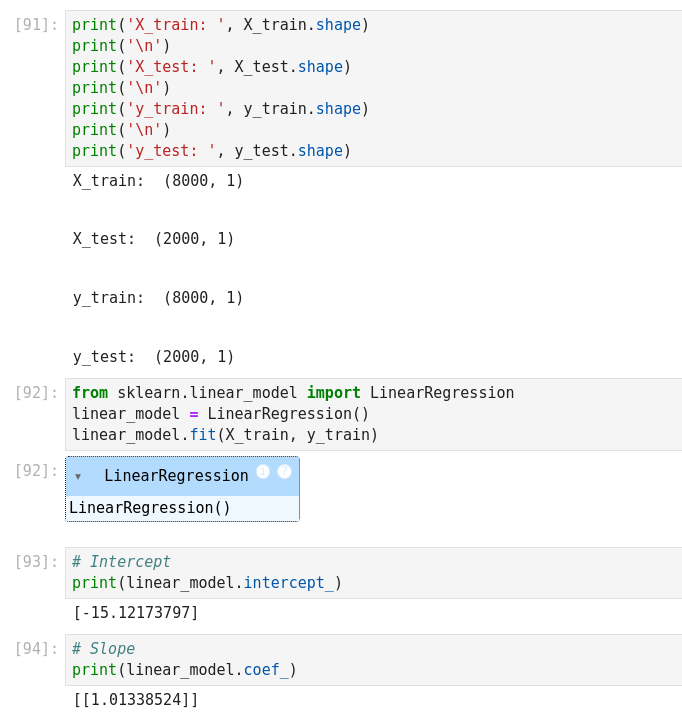
Linear regression with Scikit-Learn

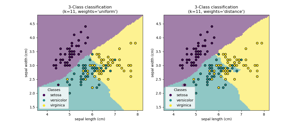
K-Nearest Neighbors (KNN) (Supervised Learning)

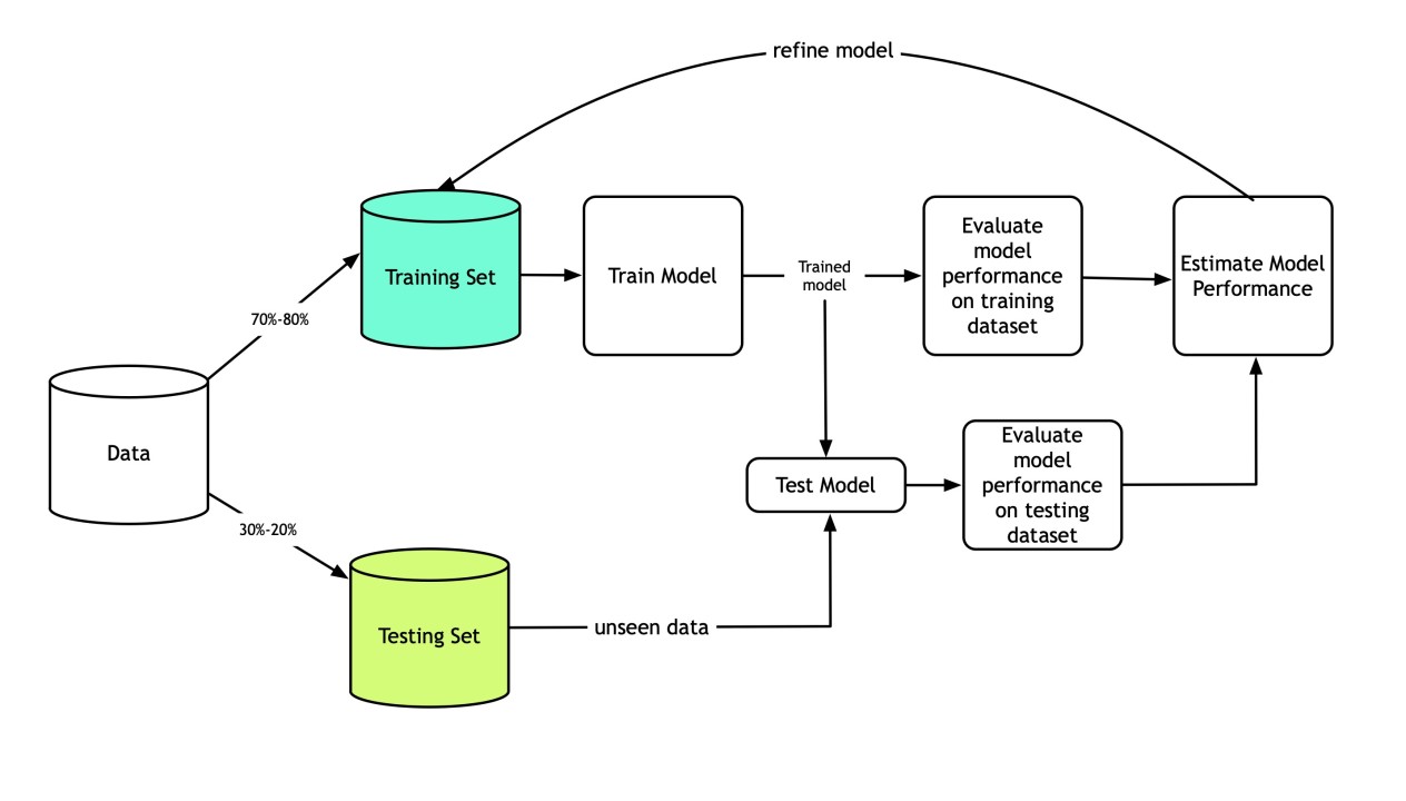
The KNN algorithm uses the entire dataset as the training set, rather than splitting the dataset into a training and test set.

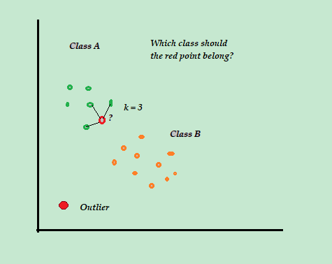
The main purpose of algorithm is to the classify the data into several classes to predict the class of new data point. The K-Nearest-Neighbor algorithm estimates how likely a data point is to be a member of one group or another.

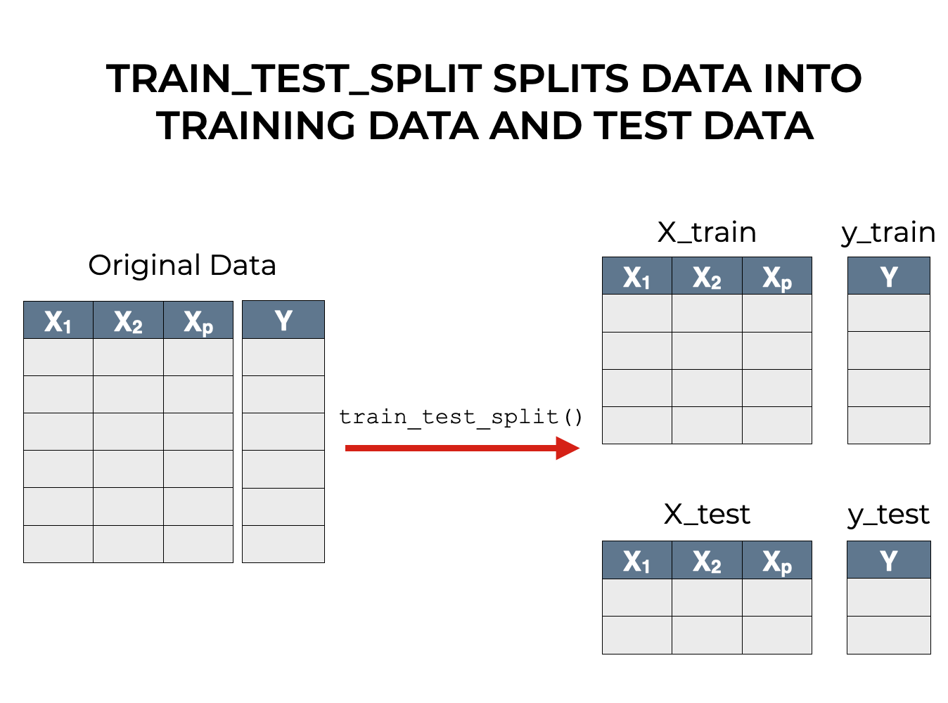
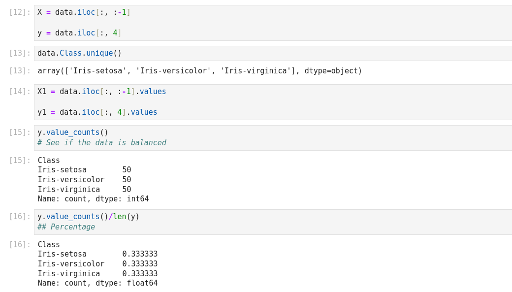
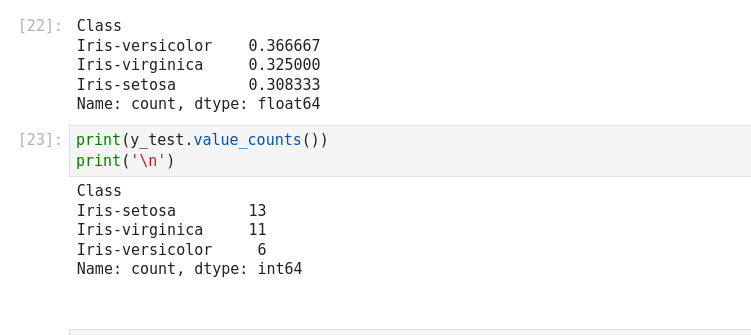
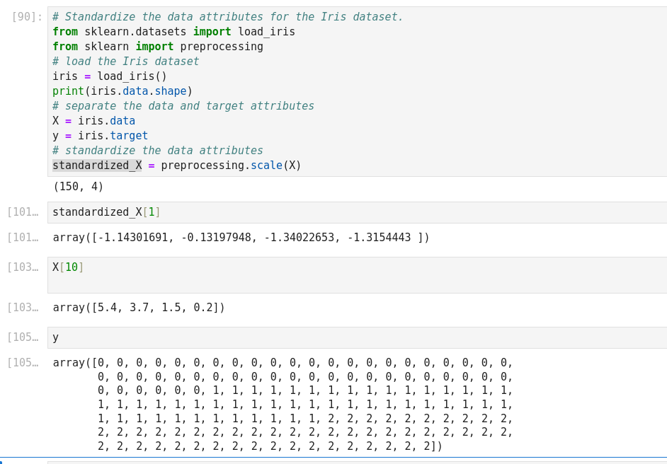
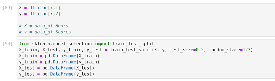
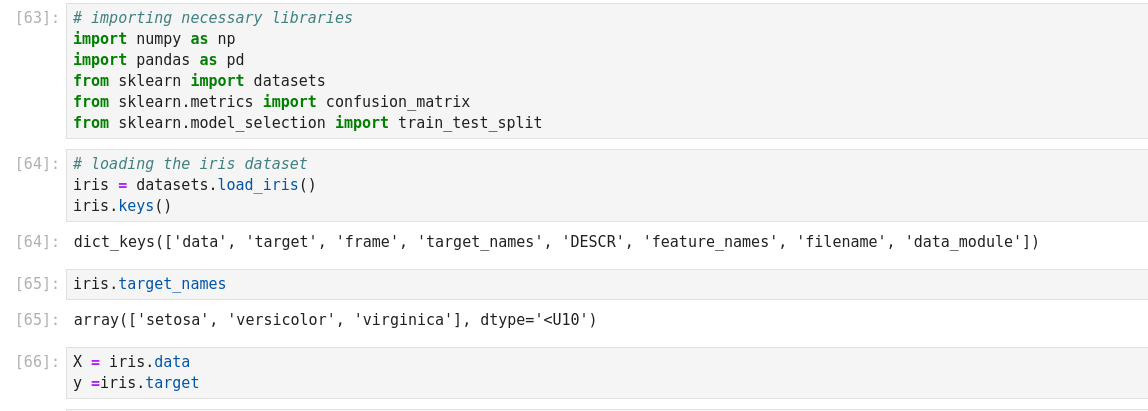
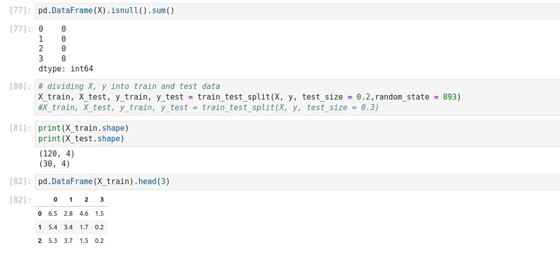
Split dataset into its input features and labels. The X variable contains the first four columns of the dataset
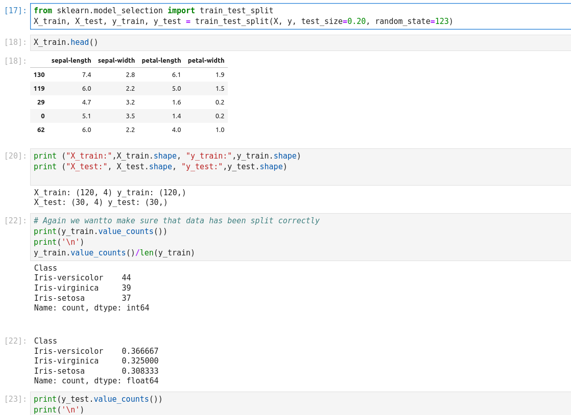
Train Test Split: deivide the data inot training and test which gives better idea as to how algorithm performed on the unseen data. The following script dived the data into 80% train data and 20% test data. (line 14)
Feature Scaling: Before making any actual predictions, it is always a good practice to scale the features so that all of them can be uniformly evaluated. (line 26)
Training and Predictions: The first step is to import the KNeighborsClassifier class from the sklearn.neighbors library. In the second line, this class is initialized with one parameter, i.e. n_neigbours. This is basically the value for the K. There is no ideal value for K and it is selected after testing and evaluation, however to start out, 3 seems to be the most commonly used value for KNN algorithm. (line 29)
The final step is to make predictions on our test data. (line32)
Evaluating the Algorithm: For evaluating an algorithm, confusion matrix, precision, recall and f1 score are the most commonly used metrics. The confusion_matrix and classification_report methods of the sklearn.metrics can be used to calculate these metrics. (line 34)
Comparing Error Rate with the K Value: In the training and prediction section we said that there is no way to know beforehand which value of K that yields the best results in the first go. We randomly chose 3 as the K value. One way to help you find the best value of K is to plot the
graph of K value and the corresponding error rate for the dataset. In this section, we will plot the mean error for the predicted values of test set for all the K values between 1 and 30. (line 39)
To plot the error values against K values. (line 40). From the output we can see that the mean error is zero when the value of the K is 2, 6, and 14. I would advise you to play around with the value of K to see how it impacts the accuracy of the predictions.
Improving kNN Performances in scikit-learn Using GridSearchCV: For deciding the value of K, plotting the elbow curve every time is a cumbersome (lourde) and tedious process. You can simply use gridsearch to find the best value. This is a tool that is often used for tuning hyperparameters of machine learning models. In your case, it will help by automatically finding the best value of K for your dataset. GridSearchCV is available in scikit-learn, and it has the benefit of being used in almost the exact same way as the scikit-learn models (line 41)

Logistic Regression (Supervised Learning – Classification)

The name “Regression” implies that a linear model is fit into the linear space. Predictions are mapped to be between 0 and 1 through the logistic function to a linear combination of feature, which means that predictions can be interpreted as class probabilities.

The goal of logistic regression is to use the train the model to find the values of coefficients such that it will minimize the error between the predicted outcome and the actual outcome.

Naïve Bayes Algorithm with Scikit

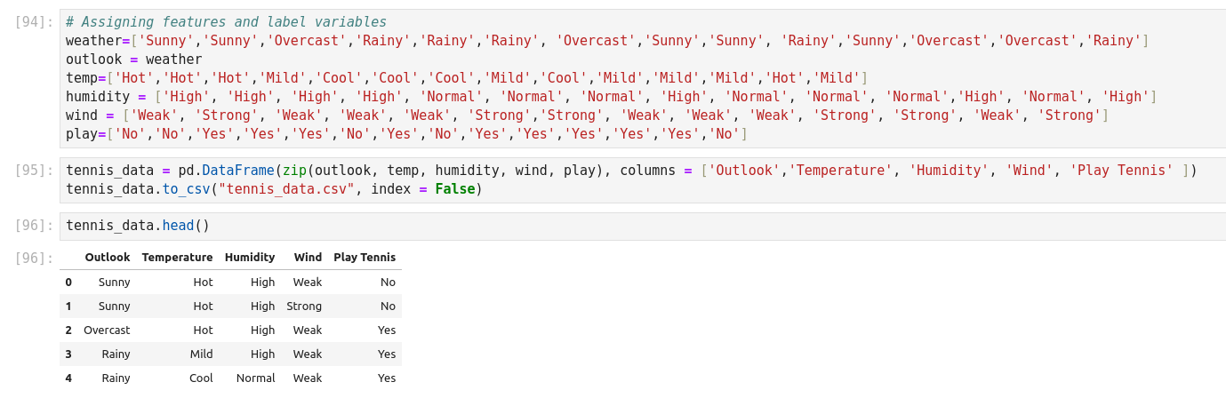
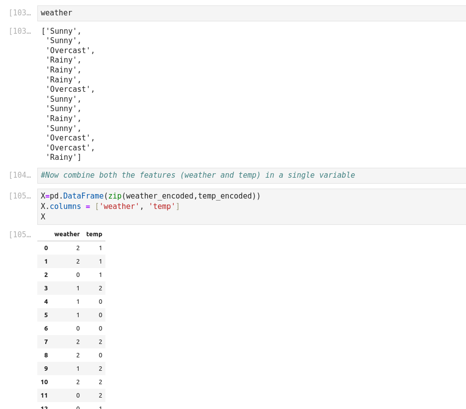
Autre exemple de Naive Bayes prediction

Cet exemple a la particularité de construire son dictionnaire, de le zipper, de l’embarquer dans un csv!

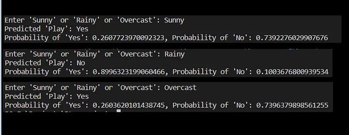
On entre les variables Weather et Temperature, et on prédit si on va jouer ou pas (play).

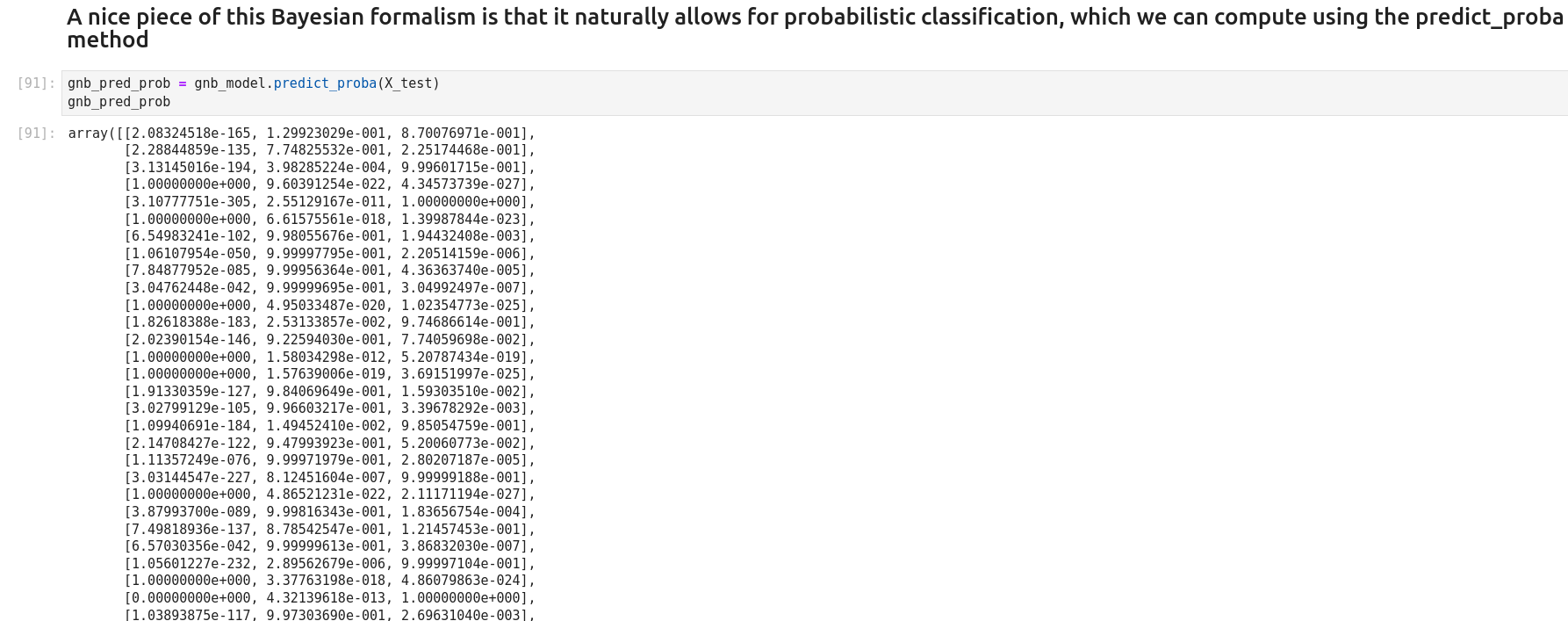
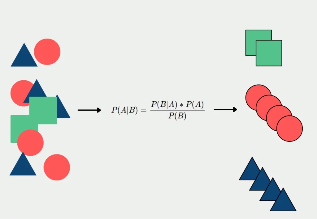
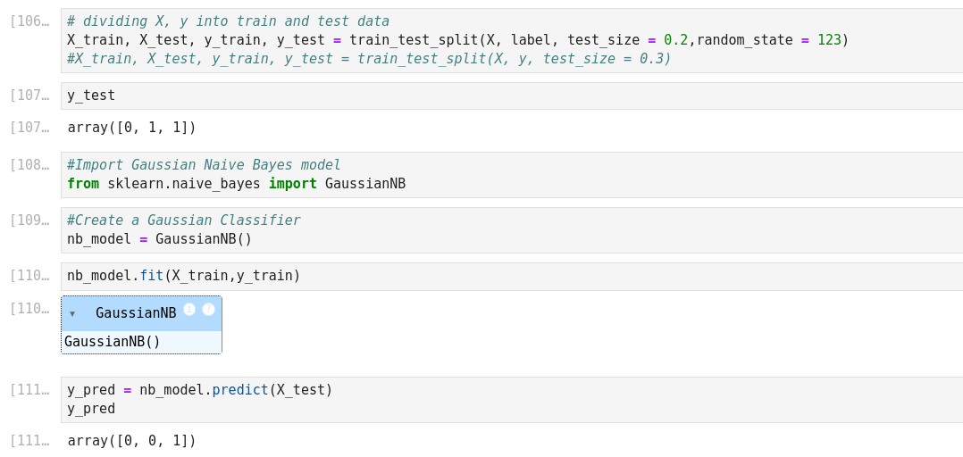
The Naive Bayes classifier is a popular and simple machine learning algorithm used for classification tasks. It is based on Bayes’ theorem, which is a probability theorem that provides a way to calculate conditional probabilities.

In a classification problem, the goal is to assign an input (or a set of inputs) to one of several predefined classes or categories. The Naive Bayes classifier works by calculating the probabilities of the input belonging to each class and then choosing the class with the highest probability as the predicted output.

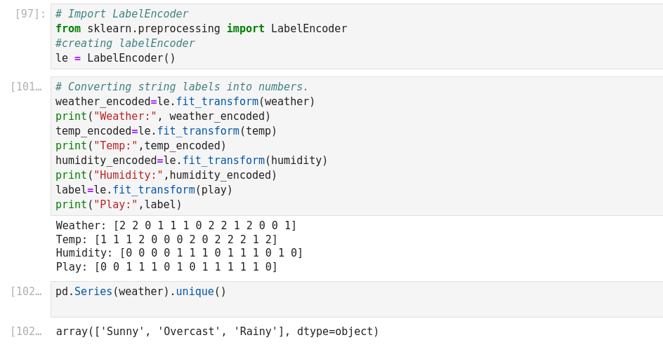
We’ll define a prediction function that takes the user’s input for the outlook (Sunny, Rainy, or Overcast) and predicts whether people will play outside or not.

Temperature: 0 = Hot >30°C, 1 = Cool (frais, < 18°C), 2=Mild (douce, 18 à 30°C)

Humidity: 0=High, 1=Normal

Windy: f=False, t=True

Play: True=1, False=0

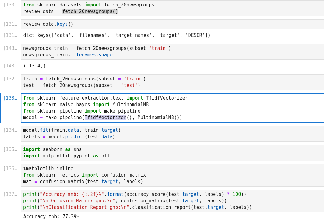
Example: Classifying Text

The 20 newsgroups dataset comprises around 18000 newsgroups posts on 20 topics split in two subsets: one for training (or development) and the other one for testing (or for performance evaluation). The split between the train and test set is based upon a messages posted before and after a specific date.

In order to feed predictive or clustering models with the text data, one first need to turn the text into vectors of numerical values suitable for statistical analysis. This can be achieved with the utilities of the sklearn.feature_extraction.text

This is a list of the 20 newsgroups:
- comp.graphics
- comp.os.ms-windows.misc
- comp.sys.ibm.pc.hardware
- comp.sys.mac.hardware
- comp.windows.x rec.autos
- rec.motorcycles
- rec.sport.baseball
- rec.sport.hockey sci.crypt
- sci.electronics
- sci.med
- sci.space
- misc.forsale talk.politics.misc
- talk.politics.guns
- talk.politics.mideast talk.religion.misc
- alt.atheism
- soc.religion.christian

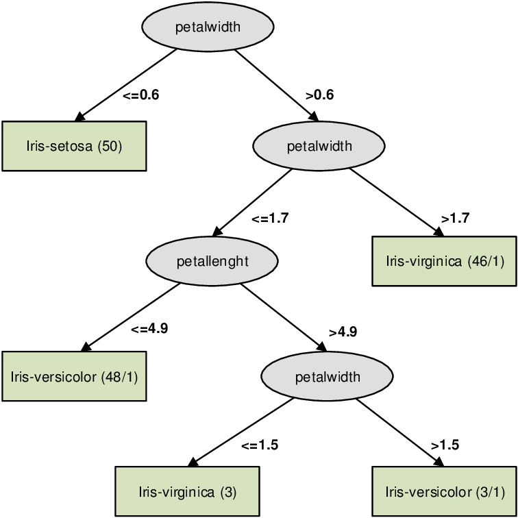
Decision Trees (Supervised Learning – Classification/Regression)

A decision tree is a flow-chart-like tree structure that uses a branching method to illustrate every possible outcome of a decision. Each node within the tree represents a test on a specific variable – and each branch is the outcome of that test. It is a graphical representation of possible solutions to a decision based on certain conditions. It’s called a decision tree because it starts with a single node
know as root node, which then branches off into a number of solutions, just like a tree. Decision tree algorithm can be used both for regression as well as classification. Decision tree method is capable of handling heterogeneous as well as missing data. Trees are further capable of producing understandable rules. The tree can be explained by two entities, namely decision nodes and leaves. The
leaves are the final outcomes and each node (decision nodes or internal nodes) within the tree represents a test on specific feature.

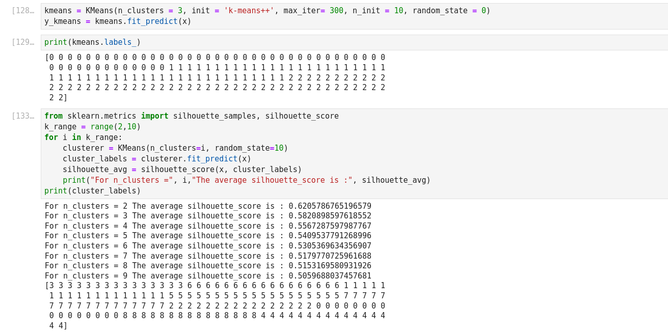
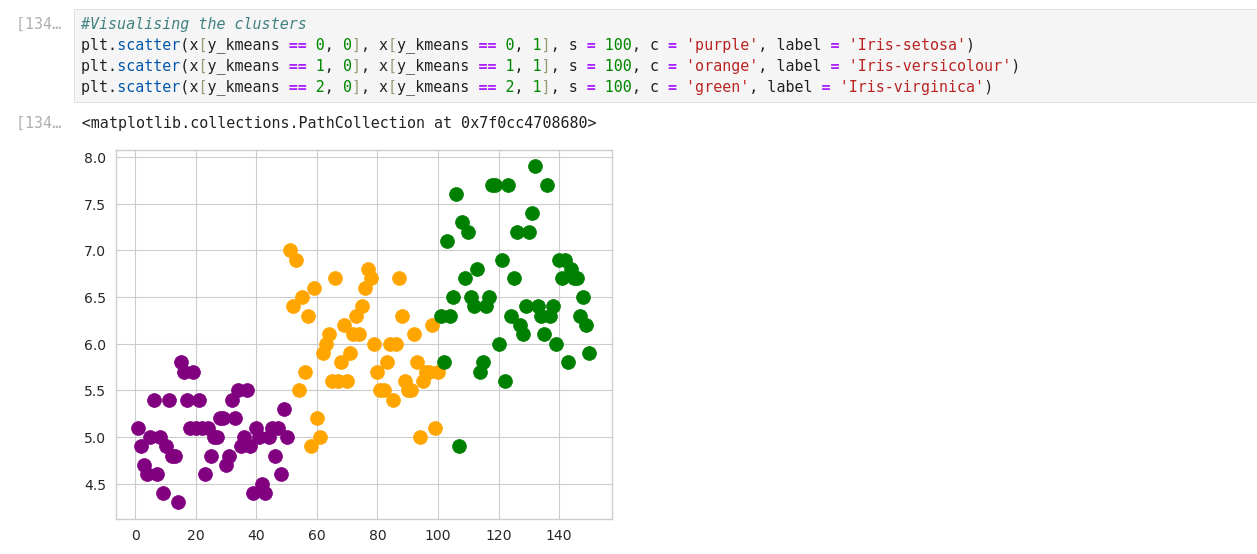
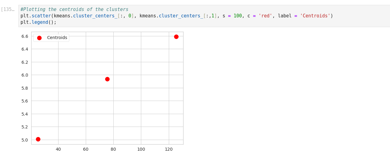
K-means Clustering with Scikit_Learn

Silhouette analysis can be used to study the separation distance between the resulting clusters. The silhouette plot displays a measure of how close each point in one cluster is to points in the neighboring clusters and thus provides a way to assess parameters like number of clusters visually.